The Singular Value Decompositions of Transformer Weight Matrices are Highly Interpretable
Please go to the colab for interactive viewing and playing with the phenomena. For space reasons, not all results included in the colab are included here so please visit the colab for the full story. A GitHub repository with the colab notebook and accompanying data can be found here.
This post is part of the work done at Conjecture.
TLDR
If we take the SVD of the weight matrices of the OV circuit and of MLP layers of GPT models, and project them to token embedding space, we notice this results in highly interpretable semantic clusters. This means that the network learns to align the principal directions of each MLP weight matrix or attention head to read from or write to semantically interpretable directions in the residual stream.
We can use this to both improve our understanding of transformer language models and edit their representations. We use this finding to design both a natural language query locator, where you can write a set of natural language concepts and find all weight directions in the network which correspond to it, and also to edit the network’s representations by deleting specific singular vectors, which results in relatively large effects on the logits related to the semantics of that vector and relatively small effects on semantically different clusters
Introduction
Trying to understand the internal representations of language models, and of deep neural networks in general, has been the primary focus of the field of mechanistic interpretability, with clear applications to AI alignment. If we can understand the internal dimensions along which language models store and manipulate representations, then we can get a much better grasp on their behaviour and ultimately may be able to both make provable statements about bounds on their behaviour, as well as make precise edits to the network to prevent or enhance desired behaviours.
Interpretability, however, is a young field where we still do not yet fully understand what the basic units of the networks’ representations are. While analyzing and investigating individual neurons has led to some impressive results, especially in convolutional vision models, a key issue has always been the polysemanticity of neurons. A single neuron might not just represent a single ‘feature’ but some linear combination of features in superposition. This effect has been studied in toy models where it is argued that neural networks resort to superposition when required to represent many more features than they have neurons, and that superposition has a regular and understandable geometry.
A natural hypothesis following from the apparent ubiquity of superposition in neural networks, as well as the autoassociative memory literature, is to store features as directions and not in individual neurons. To minimize interference ideally these directions would be pseudo-orthogonal. Technically the features as neurons hypothesis is trivially an orthogonal direction where each feature is encoded by a specific neuron, but the storage capacity of this representational scheme scales only linearly. In theory, we can do much better if we instead distribute features across multiple neurons and accept some noise. Specifically, the Johnson-Lindenstrauss lemma suggests that we can store exponentially many features in pseudorthogonal subspaces. While neural networks probably cannot utilize all of this exponential space, they almost certainly scale superlinearly, necessitating polysemanticity across ‘neurons’.
If this hypothesis is true, at least approximately, a key question becomes how we can figure out the directions in which specific features are encoded. While certainly not the entire story, we hypothesize that at least a number of the primary directions used by the network can be inferred from the SVD decomposition of its weight matrices. This makes sense since the network’s weights are ultimately linear maps that act upon its representations, and the largest singular vectors of the weight matrix are precisely the directions in which the weight matrix has the largest action. In this post, we show that these SVD directions are often highly and robustly interpretable in medium-sized transformer language models, a property we expect to apply more generally to any transformer or residual architecture.
Specifically, we demonstrate that the SVD directions of both the MLP input and output weights as well as the OV circuit in the transformer, when projected to token space, yield highly interpretable clusters for most of the singular directions. Secondly, we show that this can be applied to automatically detect weight matrices and directions in weight space that match closely with a given set of tokens, and can be used to directly edit model weights to remove or enhance specific singular directions, with strong differential effects on the output logits corresponding to those semantic directions.
Additionally, we experiment with automatic labelling of the SVD directions and find that by using GPT3 as a labeller, we can get reasonable interpretations of directions which allows us to perform comprehensive sweeps of all singular directions in the MLPs over the GPT2 model class, thus providing a proof of concept of scalable automatic labelling on a real task.
Transformer Architecture
This is a rather quick and idiosyncratic overview of the elements of transformer networks relevant to this post. You can skip or skim if you already understand a lot about transformers – i.e. if you know all the concepts in the transformer-circuits post.
For a great general tutorial on how transformers work please see this post. Here we only discuss autoregressive sequence to sequence models typified by the GPT models. We run our experiments primarily on the gpt2 series of models released by OpenAI.
Transformers learn from token sequences to token sequences. They are trained with an autoregressive objective so that they predict the next element of the sequence from the sequence prefix.
Each token in the sequence is encoded in a one-hot vector of length . These onehot token sequences are projected into the internal embedding space of dimension $ of the model through an embedding matrix so that we have .
The core of the transformer model is the residual stream so that tokens can pass through theoretically modified all the way to the end of the network. At the end, at block , the embedding representation is decoded using the transpose of the embedding matrix . This means that the embedding matrix must be approximately orthogonal.
At the end, at block . At each block information is added to the residual stream through the application of attention and MLP blocks. A single ‘block’ consists of both an attention and an MLP layer. These blocks read in the residual stream representation, perform some computation on it, and write out an output back into the residual stream. Mathematically, this results in,
Where We use insight of Elhage et al 2022 which is that we can interpret the query and key matrices and value and output matrices not as individual matrices but as single bilinear matrices and since they only implement linear maps. Following their terminology, We call these the and circuits. We are especially interested in the circuit which we will find to be highly interpretable. The matrix writes linearly into the residual stream and does not mix information between tokens while the attention circuit mixes information between tokens and is gated by the softmax nonlinearity.
The MLP layers in the transformer are simple 2 layer MLPs where is a standard activation function such as gelu. The matrix writes directly and linearly into the residual stream. The matrix reads linearly from the residual stream if you ignore the layernorm operation. The hidden layer of the MLP typically expands the dimensionality of the residual stream by a factor (which is usually 4) such that and
A transformer model consists of a large number of blocks stacked up sequentially. For instance, GPT2-medium (an approximately 300M parameter model) consists of 24 blocks.
A key insight first written about by Nostalgebraist in the logit lens is that the dimensionality of the representation is maintained exactly throughout the residual stream, and because of this we can apply the de-embedding matrix to the residual stream at any point during processing to get a sense of what the model would output if forced to stop processing at that point. This gives a sense of the way in which information is processed by the model. For instance, you can find out the block at which the model first recognizes the ‘correct’ answer to a question by projecting the activations of the residual stream at each block to token space and tracking the log-probability of the correct answer token.
A related insight recently proposed in this paper is that many of the weight matrices are of the same dimensionality as the residual stream and hence can also be projected to token space by applying the embedding matrix. For instance, the dimensionality of of the embedding is of dimension . This means that each of the columns of is of dimension which is the same dimension as the embedding and so we can multiply it by the de-embedding matrix to obtain its projection into token space. Intuitively, what this means is that for each neuron in the MLP hidden layer, we can understand how its output weight matrix tends to write back into the residual stream in terms of the tokens it primarily interacts with. They show that in some cases you can get semantic and interpretable clusters of tokens upweighted for each neuron.
However, if you play with their code you can quickly realize that their headline results are quite cherrypicked. Most neurons do not appear to encode semantically relevant dimensions in their weights, but instead appear highly polysemantic. Again, this suggests that neurons are not the right units of analysis.
Instead, we think and provide evidence that directions are a much better unit of analysis. Specifically, if instead of analyzing specific neurons—i.e. rows of the weight matrix, we perform the same analysis on the principal directions of action of the weight matrix, we obtain extremely interpretable results with high reliability and without cherrypicking. We find approximately (70-80%) of the top 50 singular vectors are highly interpretable for the later blocks of the network.
To find these principal axes of action of the matrix, we first perform a singular value decomposition of the weight matrix, and then study the singular vectors with the top-k highest singular values. Intuitively, this makes sense because the largest singular vectors encode the directions in which the action of the matrix makes the largest change to the norm of its inputs. To understand intuitively how this works, we first need to understand the singular value decomposition (SVD).
The Singular Value Decomposition SVD
You can safely skip this section if you understand the SVD.
The SVD is a well known matrix decomposition which factors a matrix into three components—matrices of left and right singular vectors, which are orthogonal, and a diagonal matrix of singular values. It can be thought of as the generalization of the eigenvalue decomposition to non-square matrices.
Mathematically, the SVD can be represented as,
Where is a rectangular matrix and is a orthogonal matrix, is a orthogonal matrix and is a diagonal matrix. We each each row of the right singular vectors and each column of the left singular vectors.
Intuitively, we can imagine the SVD as rotating the original basis to a new orthogonal basis, where the i’th singular vector quantifies the direction which has the i’th largest effect on the Frobenius norm of a random vector—i.e. the directions which the matrix expands the most. Another way to think of the SVD is that any linear transformation (encoded in a matrix) can be thought of as comprising a rotation, a rescaling, and a second rotation ‘back’ into the original basis. and can be interpreted as orthogonal rotation matrices corresponding to these rotations and the singular values can be interpreted as parametrizing this scaling. A final, helpful, intuition about the SVD is as the optimal linear compressor of a matrix with each singular vector corresponding to the ‘components’ of the matrix and the singular value to the importance of the component. It thus allows us to construct the optimal (linear) low rank approximation of a matrix by ablating the lowest singular values first.
For further intuition on how SVD works we recommend this post.
Our SVD projection method
Our method is extremely simple. Take a weight matrix of the network. Take the SVD of this matrix to obtain left and right singular vectors . Take whichever matrix has the same dimensionality as the residual stream (typically the right singular matrix ). Take the i’th component of which corresponds to the i’th singular vector Use the de-embedding matrix to project the i’th singular vector to token space . Take the top-k tokens and see that they often correspond to highly semantically interpretable clusters, which imply that this singular vector primarily acts on a semantic subspace.
Examples — analyzing the OV circuit
Here, we present some examples of applying this method to the OV circuits of GPT2-medium. If you want to look at different heads/layers please see the colab notebook.
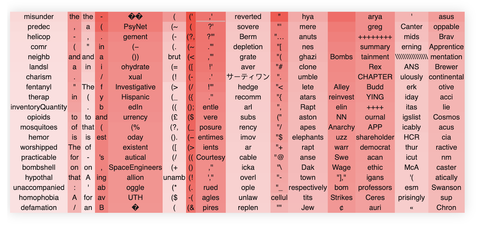
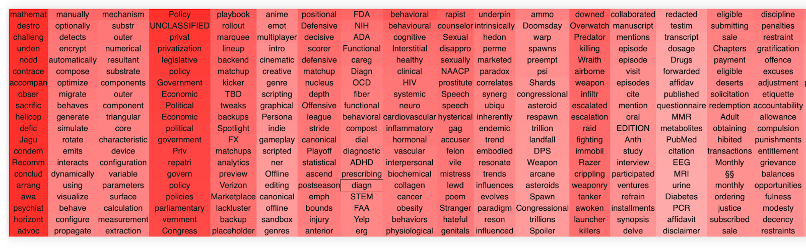
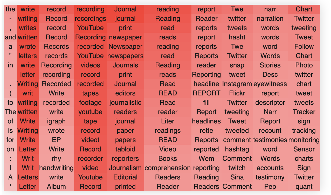
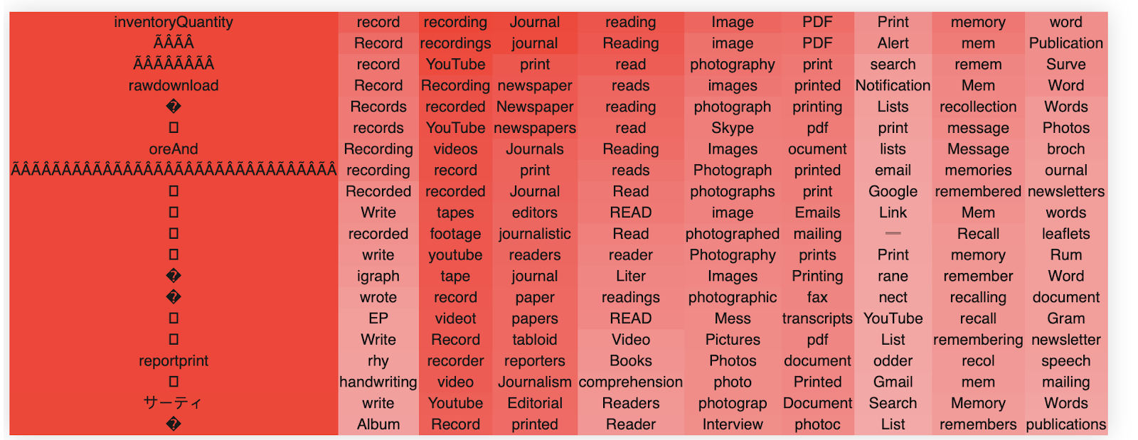
In block 22, head 10, we find these clusters. The way to read these tables is that the columns each represent a singular vector, ordered from that of the highest singular vector down to the lowest. The rows are the top-k token activations when the singular vector dimension is projected to token space, ordered by their value from top (greatest) to bottom (lowest).The colors are the strength of the embeddings.
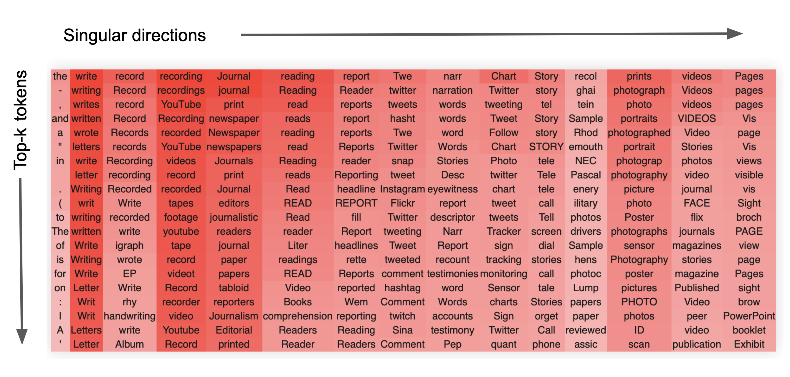
We see extremely clear semantic clusters form for each singular vector. The head as a whole clearly seems semantically related to reading/writing/literate culture and social media. We also see an interesting pattern, which is common, whereby the head as a whole seems to handle a broad concept and each singular vector specializes into a separate semantic aspect of this broader concept. For instance, in this case we see that the second singular vector specializes in writing and written things, the third and fourth in recordings and ways to record, the fifth and sixth in journals, newspapers and reading. The 7th singular vector seems closely related to social media and especially twitter, and so on.
It is very common that the first singular vector does not encode anything meaningful and simply encodes a component in the direction of the most frequent words, as in this example.
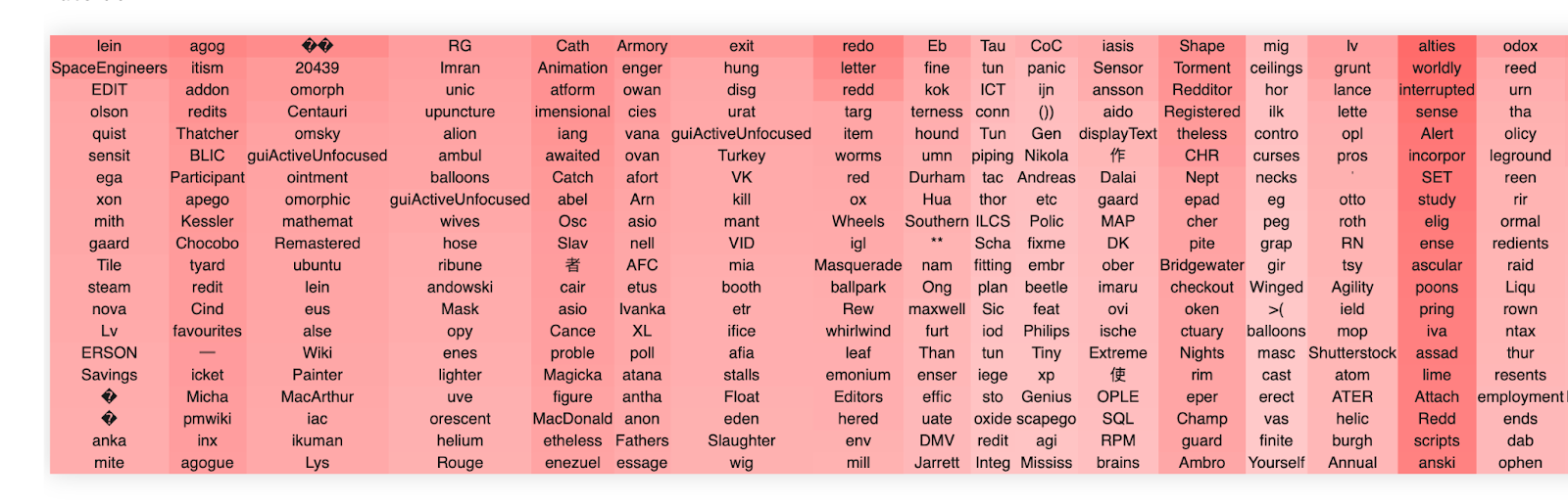
Another example is layer 22 head 15.
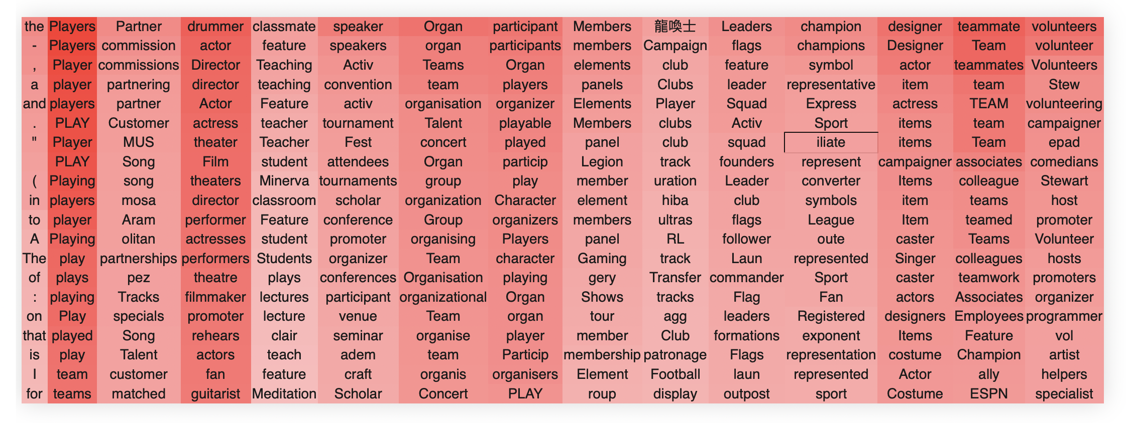
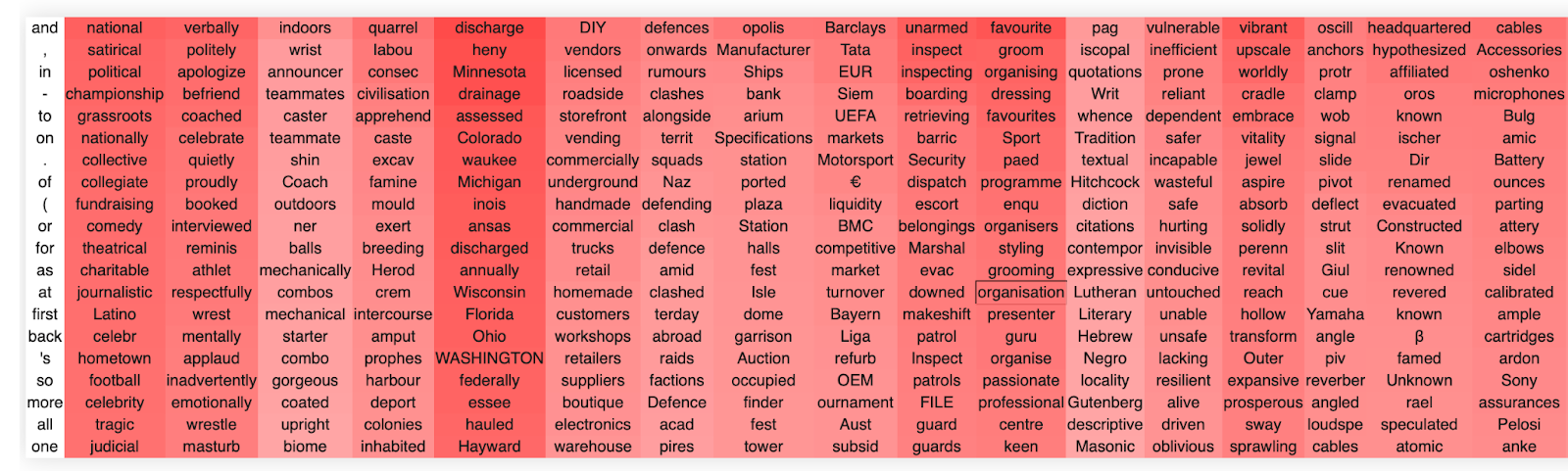
Again we see that the first singular vector encodes just some very common words. We see that this head handles a number of different concepts relating to organizations/groups but that each singular vector primarily encodes a semantically meaningful direction in this space. For instance, the second singular vector encodes playing, the third some combination of musicians, theatre, and filmmakers, the fifth organizations and teams, and so on.
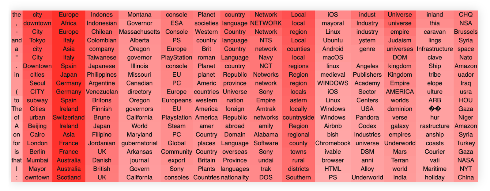
Another example of a similar direction is layer 22 head 8, which appears to encode concepts related to places, countries, cities, localities etc, although there is also a direction which clearly relates to computer operating systems.
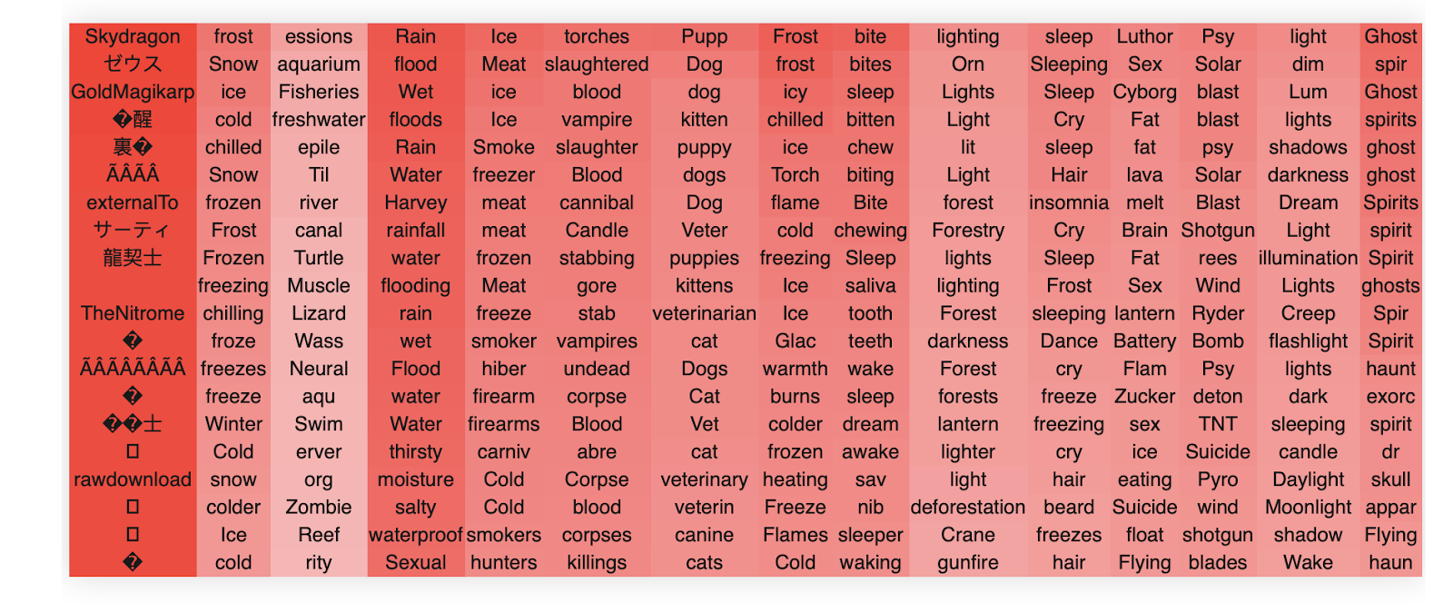
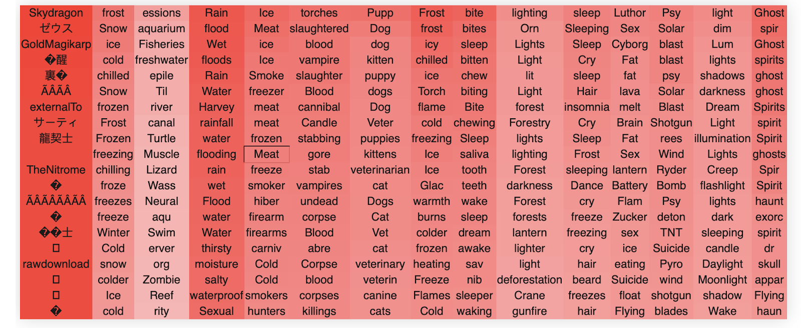
An especially interesting head is layer 22 head 3, which doesn’t appear to have a unified global semantic concept, but nevertheless many of its singular dimensions have apparently highly unrelated but clearly distinct semantic concepts, specifically frost/cold, water/rain, ice/meant/hunting/, killings/undead, dogs/animals, and so on. This head is also interesting in that its top singular vector encodes what we think are the *least* frequent tokens.
We don’t want to give the impression that all heads in the OV circuit necessarily encode nice and meaningful semantic relations. Some of them don’t appear to. For instance head 2 results in:
Some of these singular vectors clearly relate to specific punctuation patterns (this is actually a somewhat common phenomenon, especially in earlier layers) but other singular vectors appear quite uninterpretable.
We will perform a quantitative study of the fraction of interpretable layers and SVD directions later on in the post.
Finally, to show that the degree of semantic coherence we observe in the trained matrices is incredibly unlikely to occur by chance, we apply our technique to random gaussian matrices which results in entirely no semantic structure emerging at all.
If we plot the distribution of the singular vectors, we can see that the spectrum follows an approximate exponential decrease (linear on a log scale) until rank 64 when it goes to 0, since the OV matrix is only of rank 64 (the head dimension). There is also an even more rapid decline in the value of the first few singular vectors than exponential. This slow decline in log-space, gives at least some evidence towards the idea that the network is utilizing most of the ‘space’ available in this OV circuit head.
An interesting finding is that the network can encode separate information in both the positive and negative singular value directions. While each singular value is orthogona to the othersl, and hence do not interfere with each other, enabling easy and lossless superposition, the positive and negative directions are highly anticorrelated, potentially causing a significant amount of interference if it encodes two highly correlated concepts there.
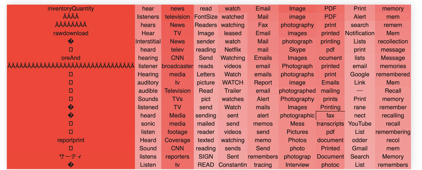
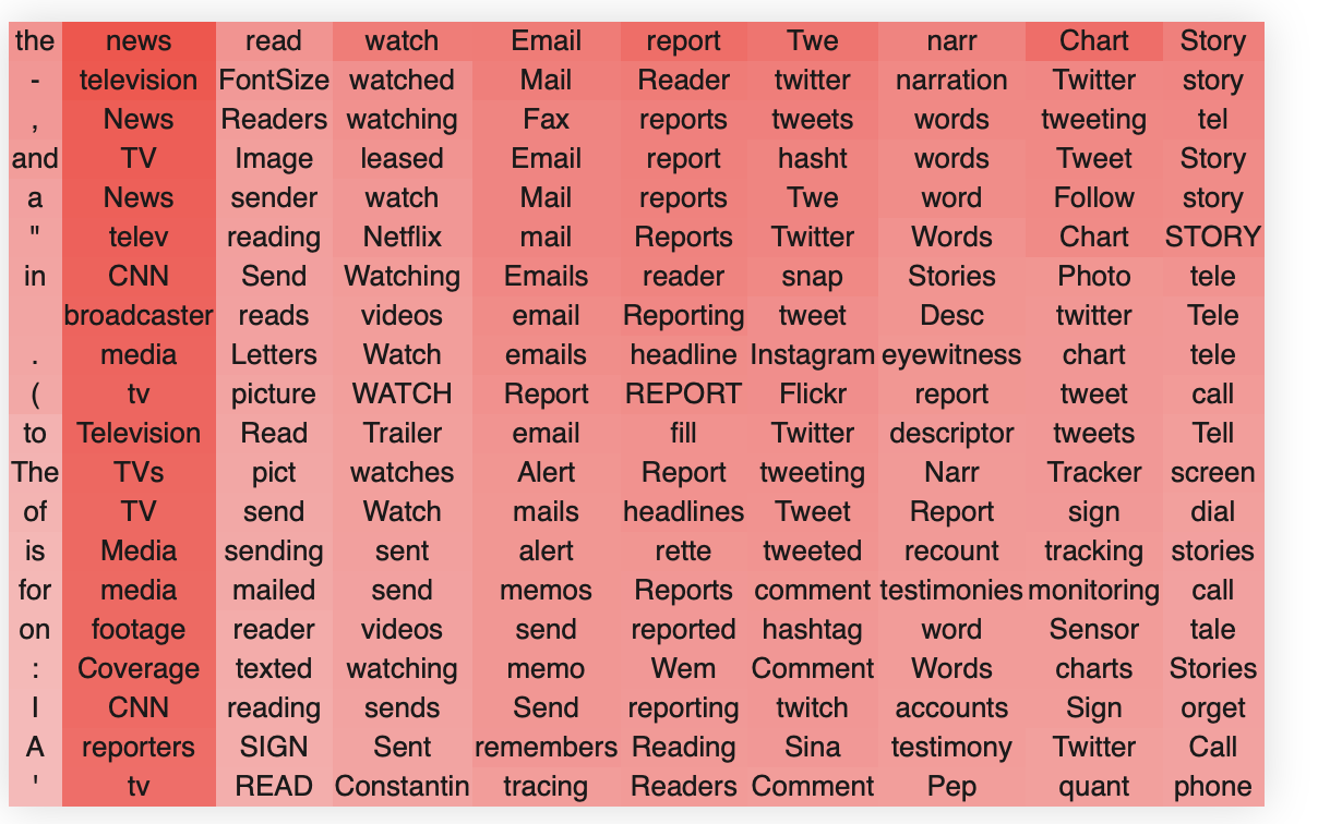
The singular value decomposition itself is ambiguous between positive and negative singular values—i.e. that we can represent a given vector as both or and get the same matrix since the two negatives cancel. This means that our labelling of positive and negative singular vectors is arbitrary, but the existence of both is not, and they can be used to encode separate information. We see that typically both the positive and negative singular values encode similar information—i.e. related to the broad concept, but often again different aspects of it. For instance, we contrast ‘hearing’ with listening in the second singular vector of this head.
It is almost always the case that the positive and negative first singular vectors are just the lists of the most or least frequent tokens encoded in an antipodal superposition.
Positive
Negative
An especially interesting phenomenon sometimes occurs where the negative and positive singular vectors encode an antipodal pair where the positive and negative are in some sense semantic opposites. This is clearly seen in head 3 where we have an antipodal encoding of fire and ice. We believe that this makes sense given that these semantic concepts are probably somewhat naturally anticorrelated resulting in little interference from putting them in superposition.
We hypothesize that, given this OV circuit writes linearly and directly to the residual stream, the existence of these antipodal directions in the weight matrix might imply the existence of such antipodal pairs in the residual stream activations. We have not yet tested this hypothesis.
MLP in interpretability
Beyond the OV circuit, we have also had significant success applying this technique to understanding the MLP layers in transformer models. This is important because thus far the MLP layers have largely resisted other analysis techniques. We can apply our projection technique of the SVD vectors to both the input and output MLP weights. This is because the SVD will always produce a matrix (whether of the left or right singular vectors) of the same shape as the embedding and does not require the weight matrices to be square.
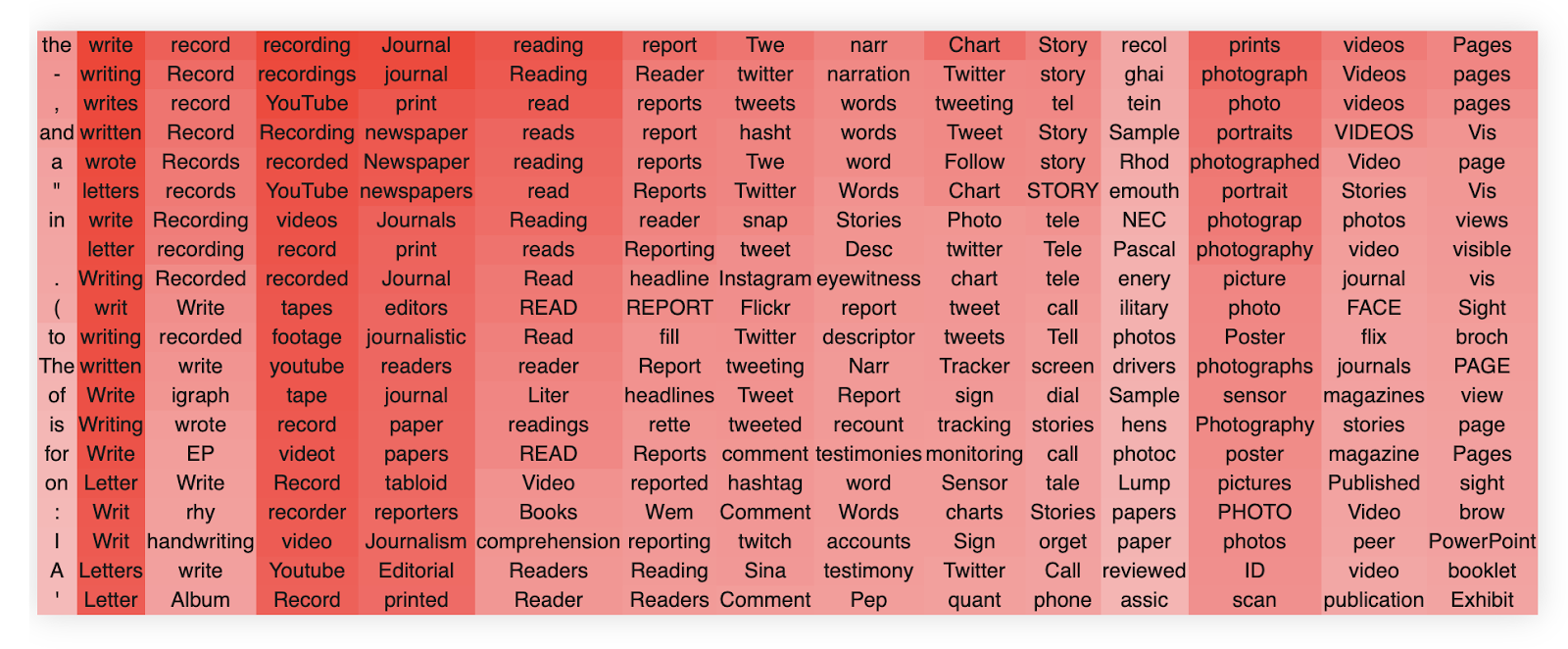
We first show that our techniques work on and then on
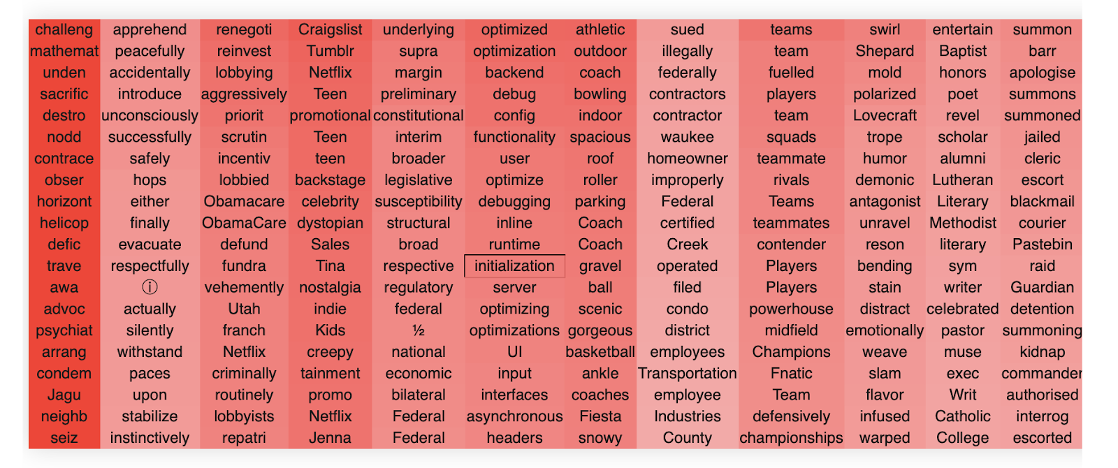
We again see that most of the singular vectors have a relatively clear semantic concept or cluster that they are referring to. For instance, singular vector 3 appears heavily related to politics, singular vector 4 to do with online businesses, and so forth.
This MLP block appears generally to have a lot of politics related words but also a wide variety of other concepts.
To get a feel for the MLPs, we plot a few more of the input weights. Unlike the attention, there is no concept of heads in MLPS, and so there are only 24 total blocks in the whole network. Thus, there is no obvious way to cherrypick.
This is layer 21 of GPT2-medium.
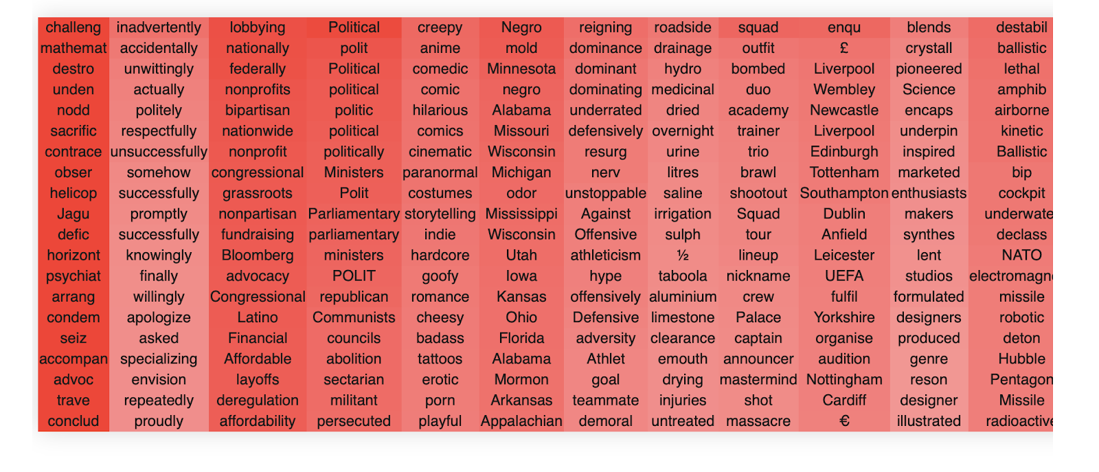
If you stare at it for a while, you begin to get a sense of how MLPs differ systematically from the OV circuits. MLPs, while each representing a single coherent concept in each singular vector, generally appear much more polysemantic than the OV circuit heads. This is probably because there is a limited amount of MLPs in the network and hence to function productively, they need to be able to represent and act on a large number of concepts simultaneously.
The MLPs also have much ‘deeper’ representations in their singular values. That is, the singular vectors are still interpretable to a much greater depth than are the attention OV circuits. This is probably because the MLP weight matrices are nearly full rank unlike the OV matrix which is low rank. This gives the network much more space to represent a wide variety of semantic concepts and the network appears to use most (but not all) of this space. Like the OV circuits, MLPs also utilize the negative singular values as additional ‘space’ to encode other semantic clusters. For instance in layer 20 we have,
Positive
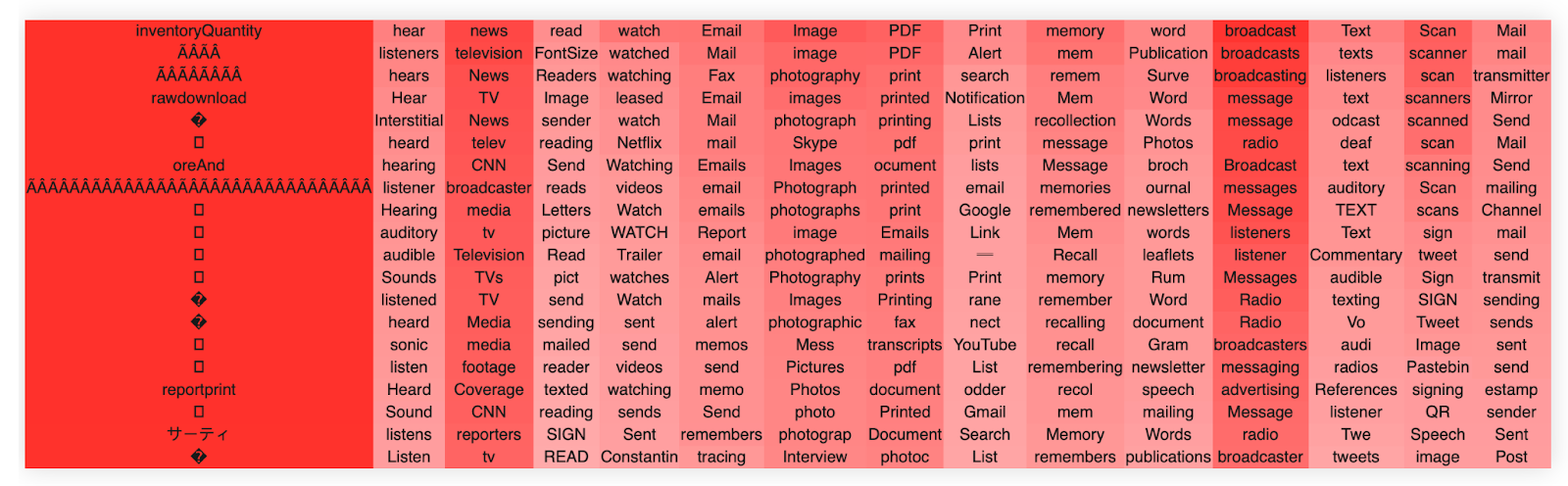
Finally, we can also apply the same approach successfully to the output weight matrix of the MLP. Overall, however, qualitatively there appear fewer super interpretable directions than . We are not entirely sure why this occurs. When we do a quantitative sweep over different models, we find this is specific primarily to GP2-medium, for reasons we are unsure about.
An example of an (layer 16) directions are
Having looked at a lot of the semantic clusters for quite a while, we have some qualitative feelings about how the different heads and MLP blocks differ from one another. However, these have not been quantitatively tested and so should not be taken as absolutely certain.
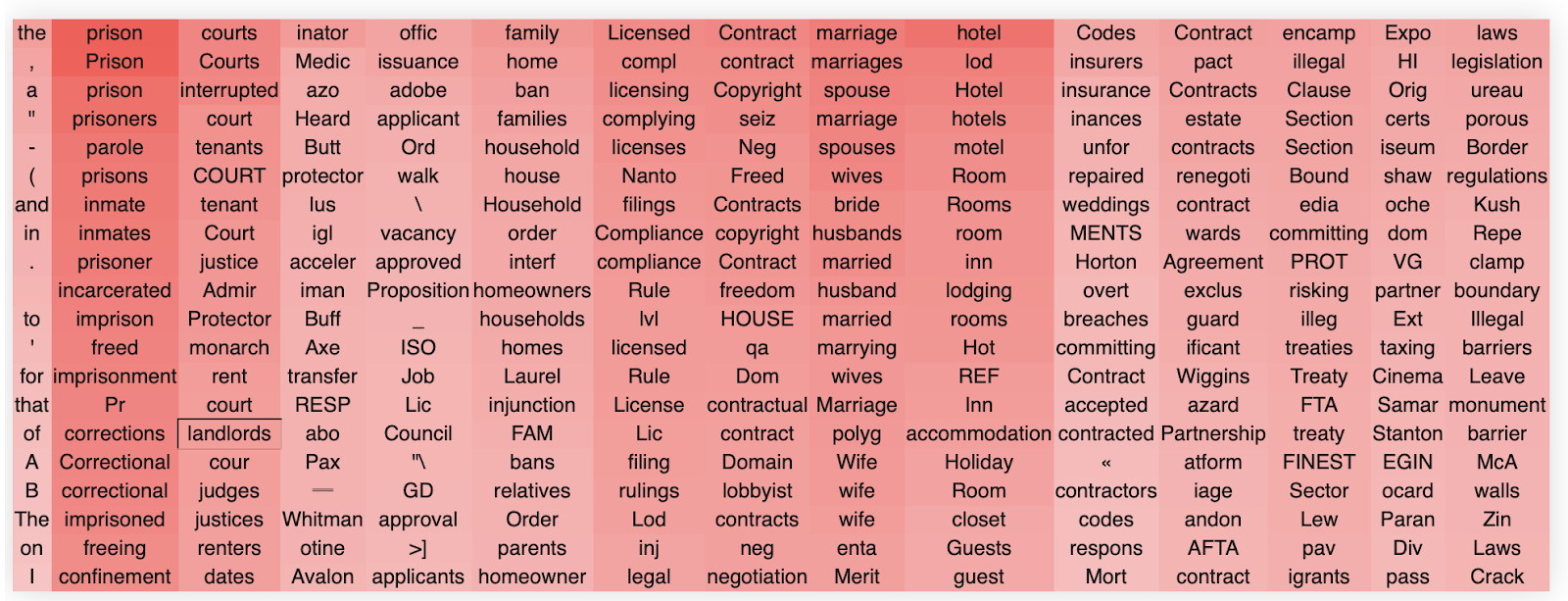
First, we find that the OV circuit heads tend to specialize in specific semantic concepts, often at quite a high level of abstraction. Then within each head, each singular value tends to represent a specialized subdirection within that broader concept. For instance, a head might represent a broad concept of something like ‘law’ and then there might be individual directions representing more specific instantiations of that concept such as lawsuits, prisons, insurance, marriages, and so forth. For instance, this is what we observe in OV circuit 19, head 5.
By contrast, the MLP blocks overall are less semantically specialized but rather tend to contain many semantically separate singular directions. This is likely because they are not organized into a specific head structure but are much larger than the independent attention heads (there being only 23 MLPs in total in the network) and they must therefore be more polysemantic. However, the singular directions themselves still tend to be extremely well separated between concepts.
The MLPs tend to have meaningful singular vectors which are much ‘deeper’ into the singular value spectrum than the OV circuit heads. I.e. that singular vectors tend to stay meaningful past the first 50 singular values while this is not the case for the OV circuits. This is unsurprising since the OV circuits are low-rank matrices since each head dimension in only 64 in GPT2-medium while the MLP weight matrices tend to be full rank. However, even in the MLP blocks, the interpretability of the singular vectors does decline significantly with depth and later MLP singular vectors (definitely by 100 or so) tend to be uninterpretable. This means either that the MLPs do not encode much semantic information beyond their first 100 singular vectors, or that our SVD token embedding projection approach cannot adequately capture this additional semantic information.
The representations also change in an interesting way with depth. As shown in our quantitative evaluation, the interpretability of each direction tends to increase with depth and peaks in the mid-to-late layers (approx 15-22) of GPT2-medium. At these late layers most of the singular vectors are highly interpretable.
What is more interesting is what happens in earlier layers. Here the interpretability of the singular vectors declines relatively smoothly with most of the singular vectors becoming uninterpretable by about layer 5. Even here, there are nevertheless a few dimensions which are highly interpretable and have as clear a semantic structure as later layers.
We hypothesize that this suggests that the network quickly forms or acts on very broad semantic clusters which can also (and perhaps more accurately) be thought of as ‘association clusters’. These can be thought of as clusters of words associated with some kind of textual domain or very broad semantic category. For instance, something like ‘words generally associated with news articles’, or ‘words generally associated with sports articles’. These can often be hard to give a strict semantic meaning to but when reading them one can often kind of see what the network is getting at.
Another thing that happens more often in earlier layers is more singular vectors dedicated to syntactic or tokenization-like processing. For instance, there are directions which respond to adverbs ending in -ly, pronouns, or other parts of speech. There are a fair number of directions which appear to respond to numbers, proper names, or various punctuation patterns. There is also a lot of directions which appear to respond to half-words with spaces before them—i.e. which have presumably been improperly split up or tokenized.
We encourage readers to play around with different layers and heads to get their own feel for the differences at different layers and between the OV circuits and the MLPs.
Manual Labelling of GPT2-medium
Because there are only a limited number of MLPs (24) in GPT2-medium it is more feasible to manually go through and look at every MLP layer and its singular vectors and manually label and count the numbers of singular vectors that are interpretable. That provides a greater and quantitative sense of the degree of interpretability provided by our approach. We sat down and manually labelled every MLP singular vector as interpretable or not in GPT2-medium.
Broadly, we set a subjective threshold of about 70-80% of tokens being aligned with a semantic direction to classify a direction as semantic. Sometimes the directions were clearly polysemantic and we did not allow these (this also implies that pure directions at least cannot be correct as a hypothesis if we have polysemantic directions!). In some cases, especially in the early layers, it was hard to make a definitive judgement as it seemed that the network had a vague idea of some cluster, but there was either a lot of noise tokens or else it was a very broad concept which was hard to justify as a specific dimension. In these cases, we erred on the side of rejecting.
If we plot the fraction of interpretable directions per block we get the following plot (shaded region is standard deviation across singular directions). We see that there is a clear increase in interpretability deeper in the network.
If we instead plot the interpretability of directions averaging across layers, we see a clear inverted U shape pattern where the first singular vector is uninterpretable (expected) while interpretability declines for later directions. Interestingly, this pattern will not be maintained in the automated approach in the next section which is a major inconsistency.
While the manually labelled data is quite noisy, several clear trends emerge. Firstly, if we plot the fraction of interpretable directions by block, we see a consistent and almost monotonic increase in the fraction of interpretable directions with depth of the block. This makes sense insofar as processing through the network should be to make information semantically relevant so as to ultimately produce a sensible output which takes into account the core semantics of language. Thus it makes sense that the later weights should be primarily acting upon interpretable (to us!) semantic subsets.
Perhaps more interesting and surprising is the singular vector distribution which roughly appears to show a U-shaped curve. The first singular values are generally not super interpretable since they tend to just respond to high (or low) frequency words and sometimes strange punctuation patterns. The middle singular vectors are often very interpretable with monosemantic clusters, and this reflects in these being the highest. As the singular vectors get smaller, they become less interpretable again, which suggests that either the network is not utilizing the space provided by these singular vectors for representations, or else that it is using them for less important and more esoteric dataset correlations that are hard for humans to understand.
From experience labelling the clusters, qualitatively, it is often correct that for some of the clusters labelled uninterpretable, it is often the case that the model is gesturing towards some kind of vague cluster you can sort of understand, but is either highly nonspecific or alternatively is clearly polysemantic.
Experiments with automated direction labelling
In the previous section, we manually hand-labelled all of the directions in the weights of GPT2-medium. However, this was a significant time commitment and is not scalable. We estimate it took about 6 hours of focused work to hand-label all of the SVD directions of the weights in GPT2-medium for 40 singular directions. At 24 MLP blocks this comes to 960 directions to label and a rate of about 3 directions a minute, which could potentially be improved but not by orders of magnitude. For larger networks and for the OV patterns where there are a large number of heads, the numbers of SVD directions rapidly become unmangeable. For instance, with 16 heads, if we wanted to label 50 SVD directions for all of the OV circuits in GPT2-medium, this would correspond to 19200 directions and about 100 hours of work. For GPT2-XL with 48 layers and 25 heads, for 50 SVD directions this comes to 60000 directions in total which would take about 330 hours to hand-label.
To get a more thorough and widespread quantitative estimate of the degree of interpretability, we experimented with automatic labelling of directions, namely asking a large language model (GPT3) to come up with potential semantic labels for each dimension, or else tell us that the dimension was not interpretable. This has the advantage of being much more scalable with the cost of being potentially noisy and biased by quirks of the labelling-LLM as well as somewhat dependent upon details of the prompt.
We experimented a lot with different prompt types including zero-shot prompting, chain of thought, and sampling approaches. We found that the model was sometimes surprisingly good at zero-shot but that it tended to reply in a number of different formats which were hard to parse automatically and it exhibited a lot of noise in its responses.
Few shot examples definitely helped the model a good deal, both in nailing down the desired response format and also in improving its accuracy at giving a sensible answer. We found that performance was highly sensitive to the number and type of few-shot examples, with often the model being strongly influenced by the relative number of positive vs negative examples (if too many positives, it invents some explanation for clearly non interpretable directions; if too many negatives, it just says that everything is uninterpretable). The model also often fixated on the few shot examples in the prompt—i.e. saying everything is about fire if there is an example of fire in the prompt. We found that performance was often non-monotonic in the number of few-shot examples and could sometimes be severely degraded by adding another few shot example.
We experimented with both the standard GPT3 model (Davinci) and the Instruct-GPT3 (text-davinci-002) models. We found the instruct model gave substantially superior performance in that it actually tended to follow the desired format and give correct answers. Davinci’s behaviour was much more variable and it especially tended to ignore the question and just invent new singular directions instead.
We tried sampling ‘best-of’ approaches and found that they did not work because the model tended to be highly certain in its answer, even clearly incorrect ones, and that this behaviour persisted at high temperatures (at super high temperatures the model’s outputs are random, and we did not manage to find a region in which the model’s outputs are relevant but high entropy). We believe this is related to the phenomenon of mode collapse in the Instruct models.
One approach to improve performance that we found worked tolerably well is to use a separate ‘verifier’ prompt, which took in both the string of direction tokens and the previous model’s outputted explanation and judge whether it was a correct interpretation or not. We found this especially useful to detect and mitigate GPT3′s tendency to make up meanings for uninterpretable directions. However, it introduced its own set of noise where sometimes the verifier model would judge some sensible interpretations to be false.
A key issue we faced was the lack of ground truth correct labels against which to judge the models’ or a prompt’s performance. We found that our own human labelled examples were often debatable and noisy also, and that sometimes we preferred the model’s judgement to our own. As such, our primary method of testing the model was to do a qualitative spot-check of the model’s performance on a set of known examples. However, this approach clearly suffers from high noise and some potential bias.
In general, despite these potential pitfalls we found that the automated labelling worked surprisingly well. GPT3 often comes up with a sensible interpretation of the singular direction, and often can find interpretations that us human labellers did not find. While not perfect as a method, we believe that it roughly captures trends in the data and gives a rough estimate of the degree of interpretability. However, the approach has high noise as well as a potential systematic bias towards saying things are more interpretable than they are, which we only somewhat corrected by the verifier model.
Ultimately our prompt consisted of a short description of the task (we found framing it as a verbal aptitude test helped the model generate relevant completions), followed by a series of few-shot examples (mostly negative to counteract the positive bias of the model). We asked the model to generate a potential semantic completion at the end. This was parsed as not-interpretable if the model said ‘these words have no semantic meaning’ and as positive if the model’s output has ‘these words’ in it, which we found a good detector of whether the model’s response is on-topic. With few-shot examples the model is very good at staying on topic and responding in the desired format.
Our verifier prompt also consisted of a short description of the task, followed by another set of few-shot examples. The model’s output was simply ‘yes’ it is a correct interpretation or ‘no’ it is not.
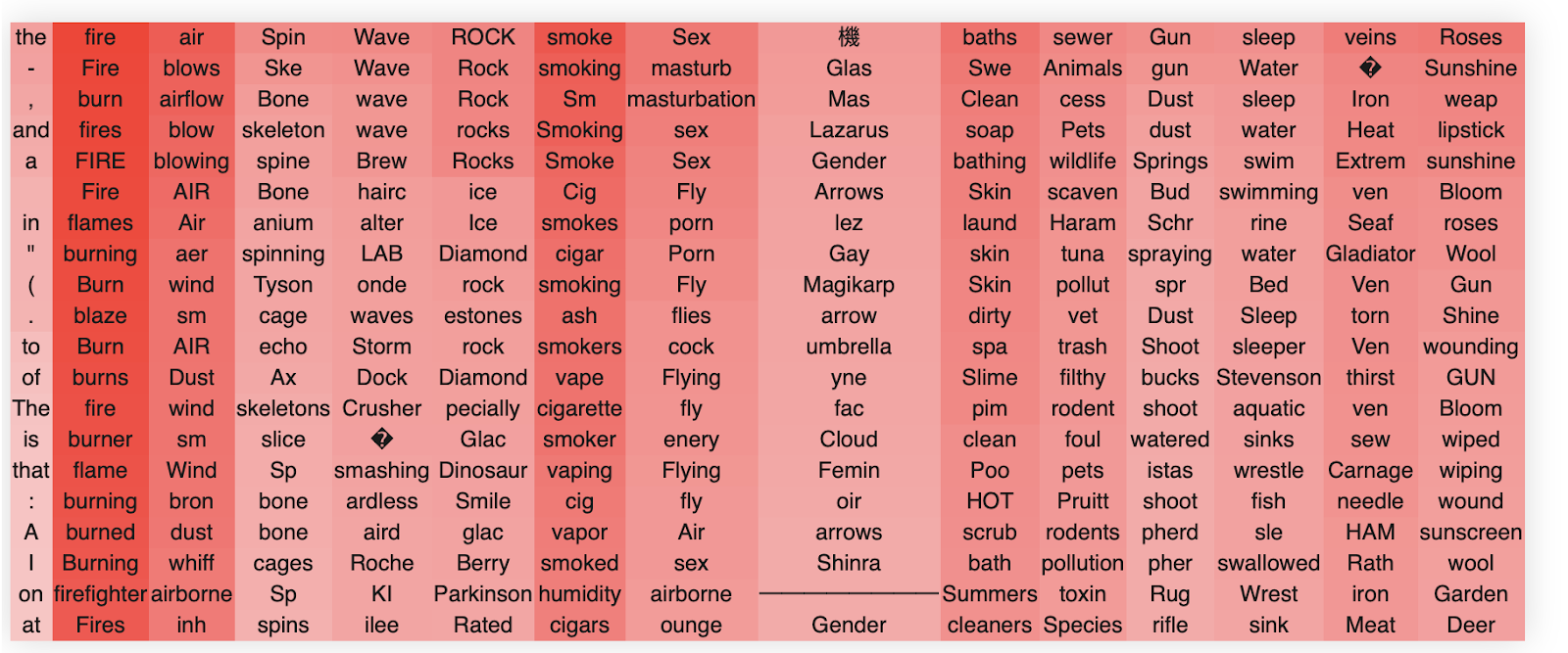
An example of the main question prompt was:
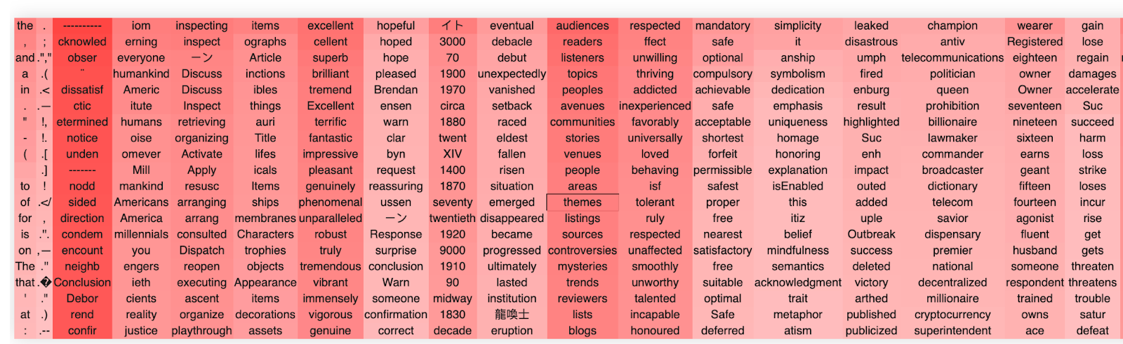
This is a transcript of the correct answers to a verbal aptitude test. The aim is to write down what semantic theme or concept a list of words has in common. A list of randomly selected correct examples is presented below in a random order.
If the words share a concept write: “most of these words are X”. If they do not share a semantic concept write: “these words have no shared semantic meaning”.
What do most of these words have in common?
the, \,, and, a, in, ., ”, -, (, to, of, for, is, on, The
Answer: most of these words are prepositions.
What do most of these words have in common?
past, oats, properties, blem, coins, enson, iliate, Alley, eatured, orial, upd, leck, hua, lat, pub
Answer: these words have no shared semantic meaning.
What do most of these words have in common?
mathemat, Iran, sophistic, methamphetamine, pty, trivia, sushi, disag, byter, etry, USB, homebrew, Mahjong, onel, Figure
Answer: these words have no shared semantic meaning.
What do most of these words have in common?
ogether, total, sole, so, otal, olute, yet, complete, all, apsed, identical, Valent, unconditional, yet, eneg
Answer: these words have no shared semantic meaning.
What do most of these words have in common?
Pupp, Dog, dog, kitten, puppy, dogs, Dog, Veter, puppies, kittens, veterinarian, cat, Dogs, Cat, Vet
Answer: most of these words relate to animals.
What do most of these words have in common?
adding, ded, strat, union, oug, vation, Tele, Strat, ould, iership, older, cium, anc, STA, secondly
Answer:these words have no shared semantic meaning
What do most of these words have in common?
The consistency check prompt was:
We are judging whether a proposed semantic interpretation of a list of words makes sense. An ideal interpretation would correctly identify a syntactic or semantic regularity among the list of words.
You will be given a question: with a list of words, and an answer with a proposed interpretation. You must answer ‘yes’ if the answer correctly identifies the syntactic or semantic commonalities of the list of words in the question, and ‘no’ otherwise.
A random list of examples is given below:
List: Pupp, Dog, dog, kitten, puppy, dogs, Dog, Veter, puppies, kittens, veterinarian, cat, Dogs, Cat, Vet
Interpretation: most of these words relate to animals.
Answer: yes
List: balloons, balloon, Wind, feather, ray, flying, Wings, FAA, ream, Wind, Winged, egg, Balloon, Render, Render
Interpretation: these words have no shared semantic meaning.
Answer: yes
List: adding, ded, strat, union, oug, vation, Tele, Strat, ould, iership, older, cium, anc, STA, secondly
Interpretation: most of these words are nouns
Answer: no
List: past, oats, properties, blem, coins, enson, iliate, Alley, eatured, orial, upd, leck, hua, lat, pub
Interpretation: most of these words are verbs
Answer: no
List: lost, missed, diminished, undone, vanished, feared, avoided, forgotten, hopeless, disappeared, fallen, removed, darkest, suspic, unavoid
Interpretation: most of these words are verbs
Answer: yes
List: mathemat, Iran, sophistic, methamphetamine, pty, trivia, sushi, disag, byter, etry, USB, homebrew, Mahjong, onel, Figure
Interpretation: these words have no shared semantic meaning
Answer: yes
List: 1 2 3
Interpretation: 4,5,6
Answer:
To run the experiment we asked GPT3 to complete these prompts for all of the first 30 singular directions for each of the MLP layers in GPT2-small, medium, and large. A direction was scored as interpretable if both the prompt model and the verifier agreed that it was. A json file containing all responses can be found and queried in the colab to get a sense of the full distribution.
If we plot the fraction of interpretable directions per block for all of the models we find:
Essentially, most blocks have a significant fraction of interpretable directions. The results are highly noisy but there does seem to be an increase with later layers being more interpretable. GPT2-medium shows the clear pattern of the MLP out layers’ interpretability peaking in the middle while the MLP in shows are more monotonic climb. A milder version of this effect (decrease in interpretability in the final layers) appears to occur in all models. We are unsure what drives this effect.
If we plot the fraction of interpretable directions found in each model of gpt2-small, medium, and large, we find a consistent pattern of the fraction of interpretable directions increasing across block size—often from about 40-50% of the directions being interpretable to about 80-90%. We see no super clear differences between the input and output MLP weights, although the data is pretty noisy so there is no clear effect. Overall, however, it is clear that across the suite of GPT2 models, a very substantial fraction of the svd directions are interpretable, showing that the results are not simply an artefact of GPT2-medium.
Interestingly, however, the effect we qualitatively observe, of the middle layers of GPT2-medium being consistently easier to interpret and the other being difficult is supported in this graph, but only for GPT2-medium. While the pattern is hard to see in GPT2-small due to the small number of blocks, in GPT2-large the pattern seems potentially extant but much less pronounced.
It is also possible to present the data in another way: plotting the fraction of interpretable blocks from each model on the same plot. Here we observe that the smaller models seem to reach roughly the same fraction of interpretable directions as the large ones, although the large ones take longer as they have more blocks.
Finally, it is also instructive to compare the fraction of interpretable directions across the singular directions themselves across all models. Here we see that a roughly consistent fraction of about 70-80% of directions are interpretable for all models, and that this does not appear to change up to 30 directions. This implies that in some sense the semanticity of the directions appears largely invariant to scaling (at least within the model scales of the GPT2 family, as well as that MLP SVD directions are ‘deep’ in that they maintain coherence up to 30 dimensions in, while the OV circuits qualitatively often start degrading around then. Clearly, to see a fall-off we need to measure more singular vectors, and were here primarily constrained by the cost of querying the OpenAI API. This is thus left to future work.
Overall, despite being highly noisy, our automated labelling approach appears to be largely consistent, but quantified our qualitative insights from before: that most SVD directions are highly interpretable, that interpretability increases in later blocks, but is always present in earlier ones, and that the MLPs are deep in their semantic meaning such that many of their singular vectors are highly interpretable. They also serve as proof of principle that automated labelling approaches work and can scale to perform comprehensive sweeps of reasonably sized models (up to a billion parameters in the GPT2 family).
SVD tracing: locating semantics with natural language prompts
While thus far we have taken a largely qualitative approach and simply looked at the semantic clusters, it would be helpful to be able to automate this approach, and specifically be able to have an automated method for locating semantic processing within the network. Specifically, it would be helpful to be able to scan a network and determine where processing of a given set of concepts is taking place.
We show that our SVD direction approach provides an initial ability to do this with a fair degree of reliability. Because we project the weight matrices to token space, we can allow querying of the weights of the network with arbitrary natural language queries and to find the weight matrix directions that most align with these queries.
The fundamental idea is that given a natural language query , we can project it to the embedding space of the network using the embedding function.
We can then simply compare the similarity of the embedding with that of the singular vectors of all of the relevant weight matrices
using a similarity function which we define as the cosine similarity. We can then compare the similarities of all the singular vectors of an MLP weight matrix or attention head and compute the top-k largest, or all of those above a threshold.
We can validate that when given queries close to the projected singular values matches with the correct singular values, and also that this method can discover new associations for a given natural language query.
For instance, we know that singular vector 1 of the OV circuit of layer 22 head 1 is associated with fire. We can find this head by inputing a bunch of fire related words into the svd trace algorithm. Interestingly, this approach also tends to return the antipodal representation—here of ‘ice/frozen’ and of ‘rain’ as well since they have strong negative cosine similarities.
For instance, for this prompt, the SVD tracing method when applied to the layer containing this singular direction gives the following result
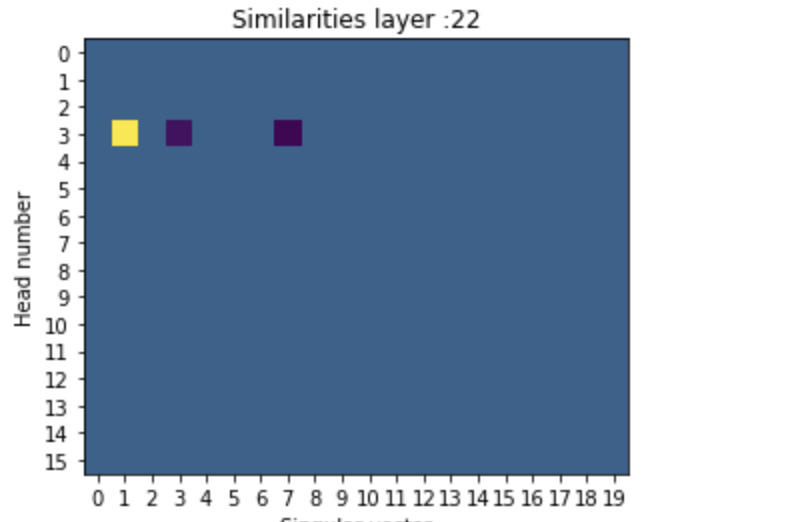
In terms of technical details, we set the threshold to 0.15 cosine similarity which we find can adequately match to the most similar representations while not including interference from other unrelated vectors. Overall, however, the translation process of embedding and de-embedding a singular vector is noisy and we can preserve only about a 0.5 cosine similarity even when utilizing the top-k tokens of a singular vector of a weight matrix directly as the query. We are unclear why this is the case and think that this method can be much improved by better similarity functions or other approaches. We also find that the embedding step is too lossy if we just use the standard embedding matrix , since it is not completely orthogonal, and that using the pseudoinverse of the de-embedding matrix works significantly better.
Directly editing SVD representations
While being able to look at and locate the semantics of individual heads or MLP blocks in terms of their singular vectors is highly useful for getting an understanding of what the network is doing, our approach also provides a preliminary way to edit the knowledge of the network. Specifically, suppose we no longer want the network to represent some SVD direction, a little linear algebra enables us to simply subtract out this direction from the weight matrix with an incredibly simple low-rank update.
Specifically, recall the matrix definition of the SVD Using the orthogonality of the singular vectors, we can break apart this matrix expression into a sum of low-rank updates,
Where is the ith singular vector, and and are the i’th columns of the left and right singular vector matrices. Given this sum, it is straightforward to see that we can a similar matrix but without this singular vector with the rank one update
Let’s see this in action. We take the layer 22, head 3 OV circuit,
Suppose we no longer like the first singular vector involving writing. We can remove this direction with a low rank update
Let’s now look at the singular vectors of the newly updated matrix. Unfortunately, the change is hard to see because due to the ambiguity of the singular vectors, when we recompute the SVD some of the positive and negative singular values can switch. We thus need to show both the positive and negative singular values to check that it has worked. Notice that all the previous singular values are still there except the first singular value about ‘writing’.
Applying these rank based updates is incredibly simple since the updates can be computed above in closed form, unlike the updates in other methods such as ROME that require an optimization process to determine the optimal updates.
We also verify that if we give the network a prompt which requires a word from the semantic cluster of a specific singular vector—in this case the ‘fire’ vector from head 3 layer 22 -- that after we apply this update, the logit of that specific token is much more highly affected than if we apply the update to the other singular vectors. This means that our updating strategy has specificity at the level of the whole network and not just of a single block. This also implicitly implies that, at least for the later blocks, the writes and reads to and from each singular vector appear to be mostly independent, or at least additive, since it is possible that later blocks can transfer information between singular vectors, thus propagating the changes induced by this method between them.
We see that when we ablate the fire vector the logprobability of outputting the word ‘fire’ to the prompt that strongly cues it decreases substantially compared to when we ablate other vectors.
Interestingly, the antipodal structure of the representations in head 3 layer 22 are on display as the logprob *increases* when we ablate singular vector 3 which is the ‘ice’ singular vector.
A key limitation of this method, however, appears to be that processing seems highly distributed through the network and that removing the singular vector from one MLP or one attention head in one block, while it has a differentially large effect on that logit, is rarely sufficient to change the global behaviour of the network. We still need to develop the targeting of multiple updates with a combined effect powerful enough to achieve targeted edits that are both specific and have large enough effect sizes to robustly and reliably change model behaviour.
However, we believe that this approach offers a promising and alternative path towards being able to make highly precise edits to existing models to sculpt their behaviour in desired ways and to remove potentially harmful information or behaviours.
Discussion
Overall, we have shown that the SVD directions of the OV and MLP-in and MLP-out weights have highly interpretable semantic directions, and that these directions can be used to selectively change model behaviour.
Returning to the more broader question over the nature of the network’s representations, we believe that the success of our method shows relatively strong support for the linear features-as-directions hypothesis, at least in residual networks. We believe this makes sense because residual networks are likely to behave in substantially more linear ways than hierarchical models such as CNNs. This is because the residual stream is a fundamentally linear mode of information transfer which is read-from and written to by linear operations. The only nonlinearities in the network occur in the residual blocks and are ‘shielded’ from the residual stream by linear transformations (if we ignore layer norms). Moreover, the ‘default’ path through the residual stream is a linear map from input to output determined solely by the embedding and de-embedding matrices meaning that if information is not written to by the nonlinear blocks, then it will remain in a linear superposition. We believe that all these factors strongly suggest that a high degree of the representational structure in the residual stream is probably linear. This is good news for interpretability, as we probably have a better hope of deeply understanding linear rather than nonlinear representations.
However, while neural networks, and especially residual architectures like transformers appear to possess a great deal of linear structure, they must also utilize a significant amount of nonlinear computation—and indeed must do so if they are to represent nonlinear functions. It is thus possible that representations are encoded in a primarily nonlinear way and our methods cannot capture these kinds of representations. Understanding the degree to which transformer representations are linear vs nonlinear, and developing methods that can help us discover, locate, and interpret nonlinear representations will ultimately be necessary for fully solving interpretability of any nonlinear neural network.
This work is also important since it begins to shed some light on the representational structure of the MLP blocks in the transformer. While some prior progress has been made on understanding the attention blocks, and specifically the attention patterns, much less progress has been made on understanding the MLP blocks. Our work is thus highly complementary to prior work in that we show that we can use our SVD directions approach to generate interpretable directions for both the MLP input and output weights, as well as the OV circuit, while our techniques have much less success when applied to the QK circuit of the attention layers. We hypothesize that this is because the processing in the QK circuit is highly syntactic as opposed to semantic. For instance, induction heads have been found in QK circuits which tend to look for tokens which follow or precede a given token and apply them elsewhere regardless of the identity of the previous token. Such a circuit would generate meaningless-looking SVD directions when projected to token space.
An important distinction to keep in mind is between the directions of representations in the activities of a network for a given input, which is the usual approach taken (i.e. in the logit lens), vs the representations of the directions of the weights. Investigating the weights has an interesting set of advantages and disadvantages compared to the activations.
A central difference which impacts the difficulty of the analysis is that the weights are static and known ahead of time while the activations can change and are technically unbounded, as an infinite number of inputs can be fed to the network resulting in different activations. Analyses of weights of a given network therefore is a promising type of static analysis for neural networks equivalent to static analysis of source code which can just be run quickly on any given network before actually having to run it on live inputs. This could potentially be used for alignment as a first line of defense against any kind of harmful behaviour without having to run the network at all. Techniques that analyze the weights are also typically cheaper computationally, since they do not involve running large numbers of forward passes through the network and/or storing large amounts of activations or dealing with large datasets.
Conversely, the downsides of weight analysis is that it cannot tell us about specific model behaviours on specific tokens. The weights instead can be thought of as encoding the space of potential transformations that can be applied to a specific input datapoint but not any specific transformation. They probably can also be used to derive information about average behaviour of the network but not necessarily extreme behaviour which might be most useful for alignment. A further line of necessary and important work will be correlating the insights we can obtain from analyzing both the weights and the activations—for instance for a given set of activations, can we trace through the primary weight directions on those activations and hence begin to get a much better sense of the true program trace of the network rather than just its static source code, which the weights provide.
Finally, while our findings of semantically interpretable SVD directions in the weights is highly robust, we believe that our applications of directly editing model weights and automated methods for finding relevant weight directions for a given query can be much improved in future work, and developing automated methods to do this will be highly important for any large scale interpretability approach. We also will try finding dataset examples that maximize the similarity with the singular vectors in the latent space, as these may give even more signal than the direct token projections.
- Critiques of prominent AI safety labs: Conjecture by (EA Forum; 12 Jun 2023 5:52 UTC; 150 points)
- Research directions Open Phil wants to fund in technical AI safety by (8 Feb 2025 1:40 UTC; 117 points)
- Deep learning models might be secretly (almost) linear by (24 Apr 2023 18:43 UTC; 117 points)
- Basic facts about language models during training by (21 Feb 2023 11:46 UTC; 99 points)
- LLM Modularity: The Separability of Capabilities in Large Language Models by (26 Mar 2023 21:57 UTC; 99 points)
- Six (and a half) intuitions for SVD by (4 Jul 2023 19:23 UTC; 73 points)
- Review of AI Alignment Progress by (7 Feb 2023 18:57 UTC; 72 points)
- ‘Fundamental’ vs ‘applied’ mechanistic interpretability research by (23 May 2023 18:26 UTC; 65 points)
- Understanding mesa-optimization using toy models by (7 May 2023 17:00 UTC; 46 points)
- EA & LW Forums Weekly Summary (28th Nov − 4th Dec 22′) by (EA Forum; 6 Dec 2022 9:38 UTC; 36 points)
- Theories of impact for Science of Deep Learning by (1 Dec 2022 14:39 UTC; 25 points)
- Understanding Counterbalanced Subtractions for Better Activation Additions by (17 Aug 2023 13:53 UTC; 21 points)
- Automatically finding feature vectors in the OV circuits of Transformers without using probing by (12 Sep 2023 17:38 UTC; 16 points)
- Critiques of prominent AI safety labs: Conjecture by (12 Jun 2023 1:32 UTC; 12 points)
- EA & LW Forums Weekly Summary (28th Nov − 4th Dec 22′) by (6 Dec 2022 9:38 UTC; 10 points)
- Spectral Taxonomy of QK Circuits in Transformer Models by (17 Oct 2025 2:18 UTC; 7 points)
- 's comment on D0TheMath’s Shortform by (19 Dec 2022 20:06 UTC; 1 point)
- 's comment on [Interim research report] Taking features out of superposition with sparse autoencoders by (3 Jan 2023 12:23 UTC; 1 point)
One subtlety which I’d expect is relevant here: when two singular vectors have approximately the same singular value, the two vectors are very numerically unstable (within their span).
Suppose that two singular vectors have the same singular value. Then in the SVD, we have two terms of the form
[u1u2][s100s1][vT1vT2]
(where the ui‘s and vi’s are column vectors). That middle part is just the shared singular value s1 times a 2x2 identity matrix:
=s1[u1u2][1001][vT1vT2]
But the 2x2 identity matrix can be rewritten as a 2x2 rotation R times its inverse RT:
=s1[u1u2]RRT[vT1vT2]
… and then we can group R and RT with U and V, respectively, to rotate the singular vectors:
=([u1u2]R)[s100s1](RT[vT1vT2])
Since UR and RTV are still orthogonal, the end result is another valid singular vector decomposition of the same matrix.
Upshot: when a singular value is repeated, the singular vectors are defined only up to a rotation (where the dimension of the rotation is the number of repeats of the singular value).
What this means practically/conceptually is that, if two singular vectors have very close singular values, then a small amount of noise in the matrix will typically “mix them together”. So for instance, the post shows a plot of singular vectors for the OV matrix, and a whole bunch of the singular values are very close together. Conceptually, that means the corresponding singular vectors are all probably “mixed together” to a large extent. Insofar as they all have roughly-the-same singular value, the singular vectors themselves are underdefined/unstable; what’s fully specified is the span of singular vectors with the same singular value.
(In fact, for the singular value distribution shown for the OV matrix in the post, nearly all the singular values are either approximately 10, or approximately 0. So that particular matrix is approximately a projection matrix, and the span of the singular vectors on either side gives the space projected from/to.)
Great point. I agree that the singular vectors become unstable when the singular values are very close (and meaningless within the span when identical). However I don’t think this is the main driver of the effect in the post. The graph of the singular vectors shown is quite misleading about the gap (this was my bad!). Because the OV matrix is effectively of rank 64, there is the sudden jump down to almost 0 which dominates the log-scale plotting. I was originally using that graph to try to show that effect, but in retrospect it is kind of an obvious one and not super interesting. I’ve replotted that graph to now cut-off at 64 and you can see that the singular values are actually reasonably spaced in log-space and roughly have an exponential decay to about 0.6. None of them are super close to their neighbours in a way that I think is likely to cause this instability.
Interestingly, the spectrums you get from doing this are very consistent across heads and you also see them in a non-truncated way in the MLP weight matrices where you see a consistent power-law spectrum.
This reminded me of some findings associated with “latent semantic analysis”, an old-school information retrieval technique. You build a big matrix where each unique term in a corpus (excluding a stoplist of extremely frequent terms) is assigned to a row, each document is assigned to a column, and each cell holds the number of times that term ti appeared in document dj , and with some kind of weighting scheme that downweights frequent terms), and you take the SVD. This also gives you interpretable dimensions, at least if you use varimax rotation. See for example pgs. 9-11 & pgs. 18-20 of this paper. Also, I seem to recall that the positive and negative singular values after doing latent semantic analysis are often both semantically interpretable, sometimes with antipodal pairs, although I can’t find the paper where I saw this.
I’m not sure whether the right way to think about this is “you should be very circumspect about saying that ‘semantic processing’ is going on just because the SVD has interpretable dimensions, because you get that merely by taking the SVD of a slightly preprocessed word-by-document matrix”, or rather “a lot of what we call ‘semantic processing’ in humans is probably just down to pretty simple statistical associations, which the later layers seem to be picking up on”, but it seemed worth mentioning in any case!
edit: seems likely that the “association clusters” seen in the earlier layers might map onto what latent semantic analysis is picking up on, whereas the later layers might be picking up on semantic relationships that aren’t as directly reflected in the surface-level statistical associations. could be tested!
Is applying SVD a new idea in interpretability? Along with “what are the eigenvalues doing”, I would have thought it was one of the basic things to study when trying to make sense of large inscrutable matrices...
Applying SVD to neural nets in general is not a new idea. It’s been used a bunch in the field (Saxe, Olah) but mostly with relation to some input data—either you run SVD on the activations, or some input-output correlation matrix or something.
You generally need to have some data to compare against in order to understand what each vector of your factorization represents exactly. What’s interesting with this technique (imo—and this is mostly Beren’s work so not trying to toot my own horn here) is twofold:
You don’t have to run your model over a whole evaluation set—which can be very expensive—to do this sort of analysis. Actually—you don’t have to do a forward pass on your model at all. Instead you can project the weight matrix you want to analyse into the embedding space (as first noted in logit lens and https://arxiv.org/pdf/2209.02535.pdf) and factorize the resulting matrix. Now you can analyse each SVD vector with regards to the model’s vocabulary, and get an idea at a glance of what kinds of processing each layer is doing. This could prove to be useful in future scenarios where e.g we want computationally efficient methods of interpretability analysis to be run during training to check for deception, or to otherwise debug a model’s behaviour.
The degree of interpretability of these simple factorizations suggests that the matrices we’re analysing operate on largely* linear representations—which could be good news for the MI field in general, as we haven’t made much headway analysing non-linear features.
*As Peter mentions below—we should avoid overupdating on this. Linear features are almost certainly low hanging fruit. Even if they represent “the majority” of the computation going on inside the network in whatever sense, it’s likely that understanding all of the linear features in a network will not give us the full story about the network’s behaviours.
Thanks for sharing this! I’m excited to see more interpretability posts. (Though this felt far too high production value—more posts, shorter posts and lower effort per post plz)
Quick feedback that the graph after this paragraph feels sketchy to me—obviously the singular values are zero beyond 64, and they’re so far low down that all singular values above look identical. But the y axis is screwed up, so you can’t really see this. What does the graph look like if you fix it? To me, it looks like there’s actually some sparsity and the early singular values are far larger (looks like there’s a big kink at the start, though it looks tiny because we’re so zoomed out).
I also personally think that a linear scale is often more principled for a spectrum graph, but not confident in that take.
Indeed, in retrospect presenting the graph this way seems to have confused a lot of people and I have now updated it to already be cut off at 64 and just show the spectrum until then, where we see a clear exponential decay in singular values (but still remaining not too small) all the way down to 64, and a slightly greater than exponential initial decay. If you want all the code is in the colab so you can set it to linear scale as well if you want. Personally I think that log-scaling tends to make more sense for spectrum graphs as they are usually exponentials or power-laws.
Indeed, we will be aiming for more rapid shorter posts in the near future. Stay tuned.
Thanks for this write-up! In case it’s of interest, we have also performed some exploratory interpretability work using the SVD of model weights.
We examine convolutional layers in models on a couple common vision tasks (CIFAR-10, ImageNet). In short, we similarly take the SVD of the weights in a CNN layer, WL=USVT, and project the hidden layer activations xl onto the ith singular vector V[i,:]xl. These singular direction “neurons” can then be studied with interpretability methods: we use hypergraphs, feature visualizations, and exemplary images. More detail can be found in The SVD of Convolutional Weights: A CNN Interpretability Framework and you can explore the OpenAI Microscope-inspired demo we created for a VGG-16 trained on ImageNet here (under the “Feature Visualization” page).
To briefly highlight a few common findings between our work and this approach, we
Also find that the top singular direction is systematically less interpretable. For the ImageNet VGG-16 model, the direction tended to encode something like a fur/hair texture, which is common across many classes. For example, see the 0th SVD neuron for the VGG-16 layers features_14, features_21, features_24, features_28 on our demo.
We find (following Martin and Mahoney) a similar distribution of singular values.
Qualitatively, the singular directions in the models we examined were at times more interpretable than neurons in the canonical basis.
And a couple questions we have:
Should we expect interpretability using the SVD of weight matrices to be more effective for transformers due to the linear residual stream (e.g., as opposed to ResNets, models without skip connections)?
There are probably scenarios where the decomposition is less appropriate. For example, how might the usefulness of this approach change when a model layer is less linear?
This is really interesting! One extension that comes to mind: SVD will never recover a Johnson-Lindenstrauss packing, because SVD can only return as many vectors as the rank of the relevant matrix. But you can do sparse coding to e.g. construct an overcomplete basis of vectors such that typical samples are sparse combinations of those vectors. Have you tried/considered trying something like that?
Yes, this is correct. SVD necessarily won’t recover the full JL packing. Given that we don’t know the extent to which the network uses the full JL capacity, then SVD might still get a reasonable fraction of the relevant directions. Also, if the network packs semantically similar vectors close to one another, then the SVD direction might also represent some kind of useful average of them.
Indeed, we are looking at sparse coding to try to construct an over complete basis, as a parallel project. Stay tuned for this.
Thank you so much for this writeup of your fascinating findings about interpreting the SVD of the weight matrix, Beren and Sid!
Completely agree. For what it’s worth, I expect interpreting nonlinear representations in complex neural nets to be quite difficult. We should expect linear-algebra methods like SVD to uncover useful information about linear representations in a straightforward manner. But we shouldn’t overupdate as a result of the ease with which linear-algebra methods uncovers this subset of information, because a lot of the relevant information is likely to pertain to nonlinear and interconnected representations, and therefore outside of this subset.
I thought this was a really good summary of the pros and cons of the methodology.
I broadly agree with this. This method definitely does not uncover any nonlinear representations in the network and is not expected to. We are primarily trying to uncover the relatively ‘easy’ information we can get with linear methods first. In further defence of linear methods, I would also argue that ‘most’ of the transformer architecture is pretty linear looking. The residual stream is linear, and the I/O matrices reading from and writing to the residual stream are also linear (if we ignore the layernorms!). I suspect that because of this some kind of linear directions might be the best way to understand representations in the residual stream, as well as writes to it, but that obviously the process of computing these writes involves nonlinear token-wise functions for the MLPs and nonlinear mixing across tokens for the attention blocks.
Looking at matrix weights through the de-embedding matrix looks interesting!
I’m unsure what kind of “matrix action” you’re hoping to capture with SVD.
In the case of symmetric square matrices, the singular directions are the eigenvectors, which are the vectors along which the matrix only multiplies them by a constant value. If the scaling factor is positive, this is what I would call “inaction”. On the other hand, even a symmetric square matrix can “stretch” vectors in interesting ways. For example, if you take (1000), I would say that the “interesting action” is not done to the singular directions (one of which is sent to zero, and the other one is kept intact), but something interesting is going on with (11) and (1−1), they both get sent to the same vector.
So I’m unsure what interesting algorithm could be captured only by looking at singular directions. But maybe you’re onto something, and there are other quantities computed in similar ways which could be more significant! Or maybe my intuition about square symmetric matrices is hiding me the interesting things that SVD’s singular directions represent. What do you think?
My bad. My intuitions about eigenvectors mislead me, and I now disagree with my comment. zfurman, on EleutherAI, gave me a much better frame to see what SVD does: SVD helps you find where the action happens in the sense that it tells you where it is read, and where it is written (in decreasing order of importance), by decomposing the transformation into a sum of [dot product with a right singular vector, scale by the corresponding singular value, multiply by the corresponding left singular vector]. This does capture a significant amount of “where the action happens”, and is a much better frame than the “rotate scale rotate” frame I had previously learned.
What does the network do if you use SVD editing to knock out every uninterpretable column? What if you knock out everything interpretable?
This is an interesting question! At the end of the post / in the colab we experiment with knocking out specific singular directions and show that it differentially affects tokens of roughly the same semantics. We find this to be quite a robust effect but that actually affecting network output can be surprisingly difficult as there seems to be large amounts of redundancy where similar processing happens in many layers/blocks simultaneously.
Knocking out every interpretable/uninterpretable column is a cool idea and we haven’t tried it. My suspicion is that this would just be too much damage to the network and would scramble things but it might be worth a shot.
I spot “GoldMagikarp” and “Skydragon”—we now know these are indeed very infrequent tokens! This was a good evidence for SolidGoldMagikarp lurking in plain sight : )
Interesting post. I just wanted to mention that your first two SVD matrix illustrations (for heads 10 and 15 of layer 22) are identical, apart from the labeled axes.
Thanks for this! This was just a copy paste error and it’s fine in the colab. Have updated the post now with the correct visuals
Should we expect these decompositions to be even more interpretable if the model was trained to output a prediction as soon as possible? (After any block, instead of outputting the prediction after the full network)
Potentially? My suspicion would be that in this case we would expect the basis in the residual stream to be extremely output-basis aligned while at the moment there is no real pressure for it to be (but it seems to be pretty output-aligned regardless, which is convenient for us). This might be a fun thing to fine-tune on.
Reminds me of [eigenwords](https://www.cis.upenn.edu/~ungar/eigenwords/) from way back when research was on word embeddings, which in makes me consider how word embedding work (Miklov etc) was like a useful precursor for interpretability in only mildly related seq2seq models (RNNs, GPTs, etc).
We’re in a similar stage of research with interpretability—many mechinterp are variations on “take a word sequence, see what activates, do it at scale, cluster the activations;” this feels somewhat analogous to BoW/Skipgram approaches for word embeddings.
seq2seq models ended up prevailing over word embedding models as they learned latent representations of words implicitly (or you might say that seq2seq was a generalization of word embeddings), which begs the question: what will the generalizations be over current activation-based mech-interp, eg probes? I think [Anthropic replacement models](https://transformer-circuits.pub/2025/attribution-graphs/methods.html) is a move that way.
More explicitly, the structural mapping is: (learn word embeddings explicitly) : (learn word embeddings latently from seq2seq) :: (learn activations explicitly) : (learn activations latently from replacement models).
Really great read. Thank you for this.
If the singular value decompositions of various matrices in neural networks is interpretable, then I suspect that various other spectral techniques that take more non-linear interactions into consideration would be interpretable as well. For research for cryptocurrency technologies, I have been investigating spectral techniques for evaluating block ciphers including the AES, but it seems like these spectral techniques may also be used to interpret matrices in neural networks as well (though I still need to do experiments to figure out how well this actually works in practice).
The singular value decomposition is designed to treat the weight matrix as a linear transformation between inner product spaces while ignoring all additional structure on the inner product spaces, so it seems like we may be able to use better spectral techniques for analyzing matrices in neural networks or other properties of neural networks since these other spectral techniques do not necessarily ignore the structure that neural networks contain. The SVD as other disadvantages including the numerical instability of the orthogonal matrices in the presence of nearby singular values, the lack of generalization to higher order tensors (higher order SVDs lose most of the interesting properties of the traditional SVD), and the inability for the SVD to find clusters of related dimensions (the top singular vectors may not have anything to do with each other so the SVD is not a clustering algorithm, and one cannot use PCA to find a cluster of dimensions). The singular value decomposition has been around since the 1800′s, so it is not exactly a cutting edge technique.
Suppose that we encode data and parameters as a collection (A1,…,Ar)∈Mn(R)r of square matrices for some r>1. Then we reduce the dimensionality of these square matrices (I call this dimensionality reduction the L2,d-spectral radius dimensionality reduction and abbreviate it as LSRDR) by finding R∈Md,n(R),S∈Mn,d(R) where RS=1d and where we maximize ρ(A1⊗RA1S+⋯+Ar⊗RArS)ρ(RA1S⊗RA1S+⋯+RArS⊗RArS)1/2 using gradient ascent where ρ denotes the spectral radius and ⊗ refers to the tensor product (the gradient process is quicker than you think even though we are using tensor products and the spectral radius). The matrices RA1S,…,RArS are the matrices of reduced dimensionality. Let P=SR. Then P2=S(RS)R=S1dR=SR=P, so P will be a projection matrix but P is not necessarily an orthogonal projection, and the vector spaces ker(P)⊥,im(P) will be clusters of dimensions in Rn. Like the singular value decomposition, the matrix P is often (but not always) unique, and this is good because when P is unique, you know that your LSRDR is well-behaved and that LSRDRs are probably a good tool for whatever you are using them for, but the non-uniqueness of P indicates that the LSRDRs may not be the best tool for whatever one is using them for (and there are other indicators of whether LSRDRs are doing anything meaningful). One can perform the same dimensionality reduction technique for any completely positive superoperator E:Mn(R)→Mn(R). We therefore need to find ways of representing parts of neural networks or parts of the data coming into neural networks as 3rd and 4th order tensors or as collections of matrices or completely positive superoperators (but the higher order tensors need to be in a tensor product of the form U⊗V⊗V or V⊗V⊗V⊗V for inner product spaces U,V in order for the LSRDR to function).
There are probably several ways of using LSRDRs to interpret neural networks, but I still need to run experiments applying LSRDRs to neural networks to see how well they work and establish best practices for LSRDRs used in interpreting neural networks.
Very interesting work! This is only a half-formed thought, but the diagrams you’ve created very much remind me of similar diagrams used to display learned “topics” in classic topic models like Latent Dirichlet Allocation (Figure 8 from the paper is below):
I think there’s possibly something to be gained by viewing what the MLPs and attention heads are learning as something like “topic models”—and it may be the case that some of the methods developed for evaluating topic interpretability and consistency will be valuable here. A couple of references:
Reading Tea Leaves: How Humans Interpret Topic Models (Chang et. al. 2009)
Machine Reading Tea Leaves: Automatically Evaluating Topic Coherence and Topic Model Quality (Lau, Newman & Baldwin, 2014)
I’d be interested in seeing other matrix factorizations explored as well. Specifically, I would recommend trying nonnegative matrix factorizations: to quote the Wikipedia article:
The added constraint may help eliminate spurious patterns: for instance, I suspect the positive/negative singular value distinction might be a red herring (based on past projects I’ve worked on).
I enjoyed reading this a lot.
I would be interested in a quantitative experiment showing what % of the models’ performance is explained by this linear assumption. For example, identify all output weight directions that correspond to “fire”, project those out only for the direct path to the output (and not the path to later heads/MLPs), and see if it tanks accuracy on sentences where the next token is fire.
I’m confused how to interpret this alongside Conjecture’s polytope framing? That work suggested that magnitude as well as direction in activation space is important. I know this analysis is looking at the weights, but obviously the weights affect the activations, so it seems like the linearity assumption shouldn’t hold?
So the quantitative experiment you propose is a good idea—and we will be working along these lines, extending the very preliminary experiments in the post about how big of an effect edits like this will have.
In terms of the polytopes, you are right that this doesn’t really fit in with that framework but assumes a pure linear directions framework. We aren’t really wedded to any specific viewpoint and are trying a lot of different perspectives to try to figure out what the correct ontology to understand neural network internals is.
I think this seems really cool. I’m excited about this. The kind of thing that I would hope to see next is a demonstration that this method can be useful for modifying the transformer in a way that induces a predictable change in the network’s behavior. For example, if you identify a certain type of behavior like toxicity or discussion of certain topics, can you use these interpretations to guide updates to the weights of the model that cause it to no longer say these types of things according to a classifier for them?
We have some preliminary results on this towards the end of the post/colab in the ‘directly editing SVD directions’ section, and are working towards improving on these currently as well as comparing to other methods such as ROME edits.
This is great!
A little while ago I made a post speculating about some of the high-level structure of GPT-XL (side note: very satisfying to see info like this being dug out so clearly here). One of the weird things about GPT-XL is that it seems to focus a disproportionate amount of attention on the first token—except in a consistent chunk of the early layers (layers 1 − 8 for XL) and the very last layers.
Do you know if there is a similar pattern of a chunk of early layers in GPT-medium having much more evenly distributed attention than the middle layers of the network? If so, is the transition out of ‘early distributed attention’ associated with changes in the character of the SVD directions of the attention OV circuits / MLPs?
I suspect that this ‘early distributed attention’ might be helping out with tasks like building multiply-tokenised words or figuring out syntax in GPT-XL. It would be quite nice if in GPT-medium the same early layers that have MLP SVD directions that seem associated with these kinds of tasks are also those that display more evenly distributed attention.
(Also, in terms of comparing the fraction of interpretable directions in MLPs per block across the different GPT sizes—I think it is interesting to consider the similarities when the x-axis is “fraction of layers through” instead of raw layer number. One potential (noisy) pattern here is that the models seem to have a rise and dip in the fraction of directions interpretable in MLPs in the first half of the network, followed by a second rise and dip in the latter half of the network.)
This seems like a super interesting result! Thanks for linking; I wasn’t aware of it. I haven’t specifically looked for this pattern in GPT2-medium but I will now! Interestingly, we have also been thinking along similar lines of a 3 phase sequence for processing in residual nets like transformers where the first few layers do some kind of ‘large scale’ reshaping process of the geometry of the data while the later layers mostly do some kind of smaller refinements which don’t change the basic geometry of the representation much, and then the final layer does one massive map to output space. This becomes quite obvious if you look at the cosine similarities of the residual stream between blocks. I hadn’t made the link with the potential attention patterns being more widely distributed at earlier layers though.
This would be easy to look at and we might see something potentially in the OV circuits. A general downside of this method is that I have never had any success with applying it to the QK circuits, and I think it’s because the attention is often performing syntactic instead of semantic operations and so projecting to embedding space is meaningless. I agree with the qualitative assessment that the early attention blocks are probably doing a lot of basic syntax/detokenization tasks like this although I don’t have a good sense of whether the MLPs are also doing this or some other kind of simple semantic processing.
I am pretty sure I made plots for this (there are definitely comparable plots in the colab already but in terms of absolute layer number instead of fraction so you will have to ‘imagine’ stretching them out. I agree there is an interesting seeming noisy pattern here. My feeling is that the early dip is probably noise and I am not sure about the later one. Definitely a lot of the time when I have qualitatively observed the final layer, the directions often suddenly become weird or meaningless in the final block.
I really appreciate this work!
I wonder if the reason MLPs are more polysemantic isn’t because there are fewer MLPs than heads but because the MLP matrices are larger—
Suppose the model is storing information as sparse [rays or directions]. Then SVD on large matrices like the token embeddings can misunderstand the model in different ways:
- Many of the sparse rays/directions won’t be picked up by SVD. If there are 10,000 rays/directions used by the model and the model dimension is 768, SVD can only pick 768 directions.
- If the model natively stores information as rays, then SVD is looking for the wrong thing: directions instead of rays. If you think of SVD as a greedy search for the most important directions, the error might increase as the importance of the direction decreases.
- Because the model is storing things sparsely, it can squeeze in far more meaningful directions than the model dimension. But these directions can’t be perfectly orthogonal, they have to interfere with each other at least a bit. This noise could make SVD with large matrices worse and also means that the assumptions involved in SVD are wrong.
As evidence for the above story, I notice that the earliest PCA directions on the token embeddings are interpretable, but they quickly become less interpretable?
Maybe because the QK/OV matrices have low rank they specialize in a small number of the sparse directions (possibly greater than their rank) and have less interference noise. These could contribute to interpretability of SVD directions.
You might expect in this world that the QK/OV SVD directions would be more interpretable than the MLP matrices which would in turn be more interpretable than the token embedding SVD.
This seems like an important but I am not sure I completely follow. How do rays differ from directions here? I agree that the SVD directions won’t recover any JL kind of dense packing of directions since it is constrained to, at maximum, the dimension of the matrix. The thinking here is then that if the model tends to pack semantically similar directions into closely related dimensions, then the SVD would pick up on at least an average of this and represent it.
I also think something to keep in mind is that we are doing the SVDs over the OV and MLP weights and not activations. That is, these are the directions in which the weight matrix is most strongly stretching the activation space. We don’t necessarily expect the weight matrix to be doing its own JL packing, I don’t think. I also think that it is reasonable that the SVD would find sensible directions here. It is of course possible that the network isn’t relying on the principal svd directions for it’s true ‘semantic’ processing but that it performs the stretching/compressing with some intermediate direction comprised of multiple SVD directions and we can’t rule that out with this method.