Six (and a half) intuitions for SVD

[CallumMcDougall]

​The long-awaited^[1] sequel to my “Six (and a half) intuitions for KL divergence” is finally here!

Thanks to the following people for feedback: Denizhan Akar, Rudolf Laine, Simon Lermen, Aryan Bhatt, Spencer Becker-Kahn, Arthur Conmy, and anonymous members of my ARENA cohort (-:

If you want to 80-20 this post (and you already know what SVD is), then just read the “Summary” section below.

Summary

The SVD is a matrix decomposition $M=US{V}^T$, where U and V are orthogonal, and S is diagonal (with non-negative diagonal elements, which we call singular values). The six intuitions are:

1. Rotations and Scalings (geometric picture)

Orthogonal matrices $U$ and $V$ can be thought of as rotations of our basis, and $S$ as a scaling of our new basis. These operations are easier to geometrically visualise than the entire operation of a matrix, with all its nuances (e.g. things like shear).

2. Best rank-$k$ Approximations

Truncating the SVD sum gives us in some sense the “best way” to approximate $M$ as a sum of rank-1 matrices. In other words, the first few matrices in the SVD sum are the “most important parts of $M$”.

3. Least Squares Regression

If we’re trying to minimize $\parallel Mx-b\parallel$ (either with a constraint on the norm of $x$ or with no constraint), we can express the solution for $x$ in terms of the SVD of $M$. When $\parallel x\parallel$ is constrained, it becomes most important to get the components of $x$ right in the directions of the largest singular values of $M$; the smaller singular values matter less.

4. Input and Output Directions (like MLPs!)

An MLP can be thought of as a collection of neurons, where each neuron has an input direction (thought of as detecting a feature) and an output direction (outputting a result if that feature is observed). ${\text{v}}_i$ and ${\text{u}}_i$ are like the input and output directions (minus the nonlinearity in the middle), and furthermore each “neuron” in this case is completely independent (orthogonal).

5. Lost & Preserved Information

SVD tells you what information (if any) is lost when you use $M$ as a linear map. It also tells you which bits of information are easier /​ harder to recover.

6A. Principal Component Analysis

If $M$ is actually a matrix of data, we can interpret the SVD matrices in terms of that data.$V$ tells you which features (= linear combinations of data) explain the most variance in the data, $S$ tells you how large this variance is, and $U$ tells you how much each datapoint is exposed to the corresponding feature.

6B. Information Compression

The Fourier transform is a popular choice of basis when compressing things like images (because with a few low-frequency Fourier basis vectors, we can usually reconstruct the image faithfully). We can think of SVD in a similar way, because it gives us the “best basis to use” for reconstructing our image, in some sense.

There are 2 key ideas running through most of these points:

• $V$ as input directions and $U$ as the corresponding output directions (i.e. we calculate $Mx$ by projecting $x$ onto the input directions, and using these projections as coefficients for our output directions)

• The SVD as being a way to efficiently represent the most important parts of the matrix, especially for low-rank matrices.

Introduction

Motivation

I’m currently doing a lot of mechanistic interpretability, and SVD is a key concept when thinking about the operations done inside transformers. Matrices like $W_{OV}$and $W_{QK}$ are very large and low-rank, making SVD the perfect tool for interpreting them. Furthermore, we have evidence that the SVD of weight matrices in transformers are highly interpretable, with the principle directions aligning with semantically interpretable directions in the residual stream.

On top of this, I think deeply understanding SVD is crucial for understanding how to think about matrices in general, and although there’s a lot of valuable stuff online, it’s not been brought together into a single resource. I hope I can do something similar with this post as I did with my KL divergence post.

Notation

Consider a matrix $M$, with size $(m,n)$. The singular value decomposition (SVD) is $M=US{V}^T$, where:

• The columns of $U$ and $V$ are orthogonal unit vectors,

• $S$ is a diagonal matrix with elements $({\sigma }_1,...,{\sigma }_r)$ where $r$ is the rank of matrix $M$, and the singular values ${\sigma }_i$ are positive & in decreasing order: ${\sigma }_1\ge {\sigma }_2\ge ...{\sigma }_r>0$.

There are a few different conventions when it comes to SVD. Sometimes it’s written with $U,S,V$ as having sizes $(m,m),(m,n),(n,n)$ respectively (in other words we pad $S$ with zeros, and fill out $U$ and $V$ with a complete basis). Alternatively, the matrices can also be written with shapes $(m,r),(r,r),(r,n)$, in other words the matrix $S$ has no zero diagonal elements. I’ll most often use the second convention, but there are times when I’ll use the first (it should be clear which one I’m using at any given time).

Lastly, note that we can also write $M$ as follows:

$$M=\sum _{i=1}^r{\sigma }_i{\text{u}}_i{\text{v}}_i^T$$

in other words as a sum of rank-1 matrices, scaled by the singular values. I claim this is the most natural way to think about SVD, and it’s the form I’ll be using for most of the rest of the post. For convenience, I’ll refer to this as the “SVD sum”.

6 ½ Intuitions

Note that there’s a lot of overlap between some of these points, and some of them cut a lot closer to the “core of SVD” than others. You might say that they’re . . . not linearly independent, and have different singular values. (I make no apologies for that pun.)

1. Rotations and Scalings (geometric picture)

Orthogonal matrices $U$ and $V$ can be thought of as rotations of our basis, and $S$ as a scaling of our new basis. These operations are easier to geometrically visualise than the entire operation of a matrix, with all its nuances (e.g. things like shear).

$U$ and $V$ are orthogonal matrices, meaning that their column vectors ${\text{u}}_i$ and ${\text{v}}_i$ are orthogonal unit vectors. We can think of them as rotations in high-dimensional space (in fact, any orthogonal matrix can be formed via a series of rotations, and possibly a reflection). $S$ is a diagonal matrix, which means it scales input along the standard basis.

The key point here is that we’re taking $M$, a general linear operation which it’s hard to get geometric intuition for, and breaking it up into a series of operations which are much easier to visualise. Let’s take possibly the simplest example of a non-trivial matrix operation: a shear.

The illustration below shows how this can be broken down as a rotation, scaling along the standard basis, then another rotation. See here for the animated version.

2. Best Low-Rank Approximations

Truncating the SVD sum gives us in some sense the “best way” to approximate $M$ as a sum of rank-1 matrices. In other words, the first few matrices in the SVD sum are the “most important parts of $M$”.

One natural way to formalise “best approximation” $M_k$ would be the matrix which minimises the value $\parallel M-M_k\parallel$, where $\parallel \cdot \parallel$ is some reasonable choice for the norm of a matrix. For example, you might use:

• The Spectral norm, $\parallel A{\parallel }_2=\underset{\parallel x{\parallel }_2\le 1}{\text{max}}\parallel Ax{\parallel }_2$

• The Frobenius norm, $\parallel A{\parallel }_F=\sqrt{{\sum }_{ij}{A}_{ij}^2}$

As it happens, the choice $M_k={\sum }_{i=1}^k{\sigma }_i{\text{u}}_i{\text{v}}_i^T$ minimises the residual $\parallel M-M_k\parallel$ for both of these norms (subject to the restriction that $M_k$ can have at most rank $k$). This is called the Eckart-Young Theorem.^[2] You can find a sketch of both proofs in the appendix.

Note—the proof relies heavily on the following lemmas:

• The spectral norm of a matrix is its largest singular value.

• The squared Frobenius norm of a matrix equals the sum of its squared singular values.

This actually hints at an important meta point in linear algebra—important concepts like Frobenius norm, trace, determinant, etc. often make a lot more sense when they’re defined in terms of the matrix when viewed as a linear map^[3], rather than when viewed as a grid of numbers. In this case, defining the Frobenius norm as the sum of squared singular values in SVD was a lot more natural than describing it as the sum of squared elements (it’s arguably easier to see how the former definition captures some notion of the “size” of the matrix). To give another example, it’s often more natural to describe the trace as the sum of eigenvalues than the sum of diagonal elements (it’s quite easy to prove the latter if you start from the former). For more on this meta point, see this section of Neel Nanda’s linear recorded algebra talk.

Key idea—the singular vectors corresponding to the largest singular values are the best way of efficiently capturing what the matrix $M$ is actually doing. If you capture most of the large singular values, then you’ve explained most of the operation of matrix $M$ (the residual linear transformation is pretty small).

3. Least Squares Regression

If we’re trying to minimize $\parallel Mx-b\parallel$ (either with a constraint on the norm of $x$ or with no constraint), we can express the solution for $x$ in terms of the SVD of $M$. When $\parallel x\parallel$ is constrained, it becomes most important to get the components of $x$ right in the directions of the largest singular values of $M$; the smaller singular values matter less.

Firstly, let’s take the least squares expression:

$$\begin{array}{c}\underset{\text{x}}{min}\parallel M\text{x}-\text{b}{\parallel }_2^2\end{array}$$

and substitute in the singular value decomposition of $M$. Spectral norm is unchanged when you perform unitary maps, so:

$$\parallel M\text{x}-\text{b}{\parallel }_2=\parallel US{V}^T\text{x}-\text{b}{\parallel }_2=\parallel S{\text{x}}_v-{\text{b}}_u{\parallel }_2$$

where:

• ${\text{x}}_v=V^T\text{x}$ are the components of $\text{x}$ in the basis created from the columns of $V$

• ${\text{b}}_u=U^T\text{b}$ are the components of $\text{b}$ in the basis created by columns of $U$

When written in this form, we can read off a closed-form expression for the solution:

$$x_{v_i}=\{\begin{array}{cc}{b}_{u_i}/{\sigma }_i& \text{if}{\sigma }_i>0\\ \text{doesn't matter}& \text{else}\end{array}$$

where $x_{v_i}=({\text{x}}_v{)}_i$ is the component of $\text{x}$ along the $i$-th column of $V$, and $b_{u_i}=({\text{b}}_u{)}_i$ is the component of $\text{b}$ along the $i$-th column of $U$. This result suggests the following terminology^[4], which we’ll use from here on out:

• the columns of $V$ are the input directions of the matrix $M$,

• the rows of $U$ are the corresponding output directions.

The problem of least squares regression then reduces to a simple one: make sure the components of $x$ along the input directions match up with the corresponding target output directions.

What about constrained optimization? Suppose we were trying to minimize $\parallel M\text{x}-\text{b}{\parallel }_2^2$ subject to the restriction $\parallel \text{x}{\parallel }_2\le m$. We can write the solution in this case as ${\text{x}}_{v_i}=\frac{1}{{\sigma }_i+\lambda /{\sigma }_i}{\text{b}}_{u_i}$, where $\lambda$ is the smallest possible non-negative real number s.t. $\parallel \text{x}{\parallel }_2\le m$.^[5] Note that, the larger the singular values ${\sigma }_i$ are, the closer our coefficient $\frac{1}{{\sigma }_i+\lambda /{\sigma }_i}$ is to the “unconstrained optimal value” of $1/{\sigma }_i$. In other words, the larger singular values are more important, so in a constrained optimization we care more about the components of $\text{x}$ along the more important input directions ${\text{v}}_i$.^[6]

A general point here—least squares isn’t an easy problem to solve in general, unless we have SVD—then it becomes trivial! This is a pretty clear sign that SVD is in some sense the natural form to write a matrix in.

4. Input and Output Directions (like MLPs!)

An MLP can be thought of as a collection of neurons, where each neuron has an input direction (thought of as detecting a feature) and an output direction (outputting a result if that feature is observed). ${\text{v}}_i$ and ${\text{u}}_i$ are like the input and output directions (minus the nonlinearity in the middle), and furthermore each “neuron” in this case is completely independent (orthogonal).

As we touched on in the previous point, the columns of $V$ can be thought of as input directions for $\text{x}$, and the columns of $U$ are the output directions. This is actually quite similar to how MLPs work! A simple MLP (ignoring biases) is structured like this:

$$MLP\left(\text{x}\right)=W^{out}f\left(W^{in}\text{x}\right)$$

where $f$ is a nonlinear function which acts element-wise (e.g. ReLU) and $W^{in}$, $W^{out}$ are the input and output weight matrices respectively. We can write this as a sum over neurons:

$$MLP\left(\text{x}\right)=\sum _{i=1}^{d_{mlp}}f(W_{[i,:]}^{in}\cdot \text{x})W_{[:,i]}^{out}$$

in other words, each neuron $i$ has an associated input direction $W_{[i,:]}^{in}$ and an output direction $W_{[:,i]}^{out}$, and we get the output of the MLP by projecting $x$ along the input direction, ReLUing the results, and using this as our coefficient for the output vector.

Compare this to SVD. We can write $M=US{V}^T={\sum }_{i=1}^r{\sigma }_i{\text{u}}_i{\text{v}}_i^T$, so we have:

$$M\text{x}=\left(\sum _{i=1}^r{\sigma }_i{\text{u}}_i{\text{v}}_i^T\right)\text{x}=\sum _{i=1}^r\left({\sigma }_i{\text{v}}_i^T\text{x}\right){\text{u}}_i$$

in other words, we calculate the output of $x$ when put through the linear map $M$ by projecting it along each of the input directions $v_i$, multiplying by scale factors ${\sigma }_i$, and using this as our coefficient for the output vector $u_i$.

The main differences between SVD in this form and MLPs are:

• MLPs are nonlinear thanks to their ReLU function. SVD is entirely linear.

• In MLPs, it’s common to have more neurons than dimensions of the input (e.g. in transformers, we usually have 4x more). This means some pairs of neurons are certain to have non-orthogonal input or output directions. In contrast, not only does SVD have $r\le \text{dim}\left(\text{x}\right)$, but every pair of input and output directions is guaranteed to be orthogonal. Furthermore, if most singular values are zero (as is the case for large low-rank matrices like $W_{OV}$), then $r$ will be much smaller than $\text{dim}\left(\text{x}\right)$.

These two points help explain why we might expect the SVD of the transformation matrices $W_{OV}$ to be highly interpretable. Note that we can also view SVD as a way of trying to tackle the “lack of privileged basis” problem—just because the standard basis isn’t privileged doesn’t mean there can’t exist directions in the space which are more meaningful than others, and SVD can be thought of as a way to find them.

5. Lost & Preserved Information

SVD tells you what information (if any) is lost when you use $M$ as a linear map. It also tells you which bits of information are easier /​ harder to recover.

For any vector $\text{x}$, we can write $\text{x}=V\text{y}={\sum }_i{y}_i{\text{v}}_i$ (where ${\text{v}}_i$ are the columns of $V$). Then, we have:

$$M\text{x}=US{V}^T\text{x}=US{V}^{T}V\text{y}=US\text{y}=\sum _i{\sigma }_i{y}_i{\text{u}}_i$$

So the singular values ${\sigma }_i$ tell how much we scale the component of $\text{x}$ in the $i$-th input direction ${\text{v}}_i$. If ${\sigma }_i=0$ then that component of $\text{x}$ gets deleted. If ${\sigma }_i$ is very close to zero, then that information gets sent to very-near-zero, meaning it’s harder to recover in some sense.

This is why doing line plots of the spectra for transformer weight matrices can be quite informative. Often, the largest singular values will dominate, and the rest of them will be pretty small. Take the example below, of the size (1024, 768). Even though the rank of the matrix is technically 768, we can see from the singular values that the matrix is “approximately singular” after a much smaller number of singular values.

SVD of GPT2-small

Another way of describing this concept is with pseudo-inverses. We say that matrix $N$ is a left-inverse of $M$ if its shape is the transpose of $M$, and $NM=I$. If this is impossible (e.g.$M$ has size $(m,n)$ with $m<n$) then we can still choose $N$ to get as close as possible to this:

$$NM=\left[\begin{array}{cc}{I}_r& 0\\ 0& 0\end{array}\right]$$

In this case, we call $N$ the “pseudo left-inverse” of $M$.

What does this look like in SVD? If $M=US{V}^T$ (where $S$ is the version with all positive diagonal values), then we have $N=V{S}^{-1}{U}^T$ as our pseudo left-inverse. We can see that, for singular values ${\sigma }_i$ close to zero, $N$ will be in danger of blowing up.

6A. Principal Component Analysis

If $M$ is actually a matrix of data, we can interpret the SVD matrices in terms of that data.$V$ tells you which features (= linear combinations of data) explain the most variance in the data, $S$ tells you how large this variance is, and $U$ tells you how much each datapoint is exposed to the corresponding feature.

Suppose $M$ is a matrix of (centered) data, with size $(n,p)$ - i.e. there are $n$ datapoints, and each datapoint has $p$ features. The rows are the datapoints, the columns are the feature vectors. The empirical covariance matrix is given by $\Sigma =\frac{1}{n-1}{M}^{T}M$, i.e.${\Sigma }_{ij}$ is the estimated covariance of features $i$ and $j$ in the data. When writing this in SVD, we get:

$$\Sigma =\frac{1}{n-1}\left(US{V}^T{)}^T\right(US{V}^T)=\frac{1}{n-1}V{S}^2{V}^T$$

This is just $S^2$ with respect to the basis of $V$. Conclusion—the columns of $V$ (which we also call the principal components) are the directions in feature space which have the highest variance, and the (scaled) squared singular values are that variance. Also, note that $V^T\Sigma V$ is a diagonal matrix (with diagonal entries $\frac{{\sigma }_i^2}{n-1}$); this tells us that the “singular features” found in $V$ have zero covariance, i.e. they vary independently.

How does $U$ fit in here? Well, ${\text{u}}_i=\frac{1}{{\sigma }_i}M{\text{v}}_i$, so each element of the vector ${\text{u}}_i$ is the dot product of a row of data with the feature loadings for our $i$-th “singular feature” (scaled by the standard deviation of that feature). From here, it’s not a big leap to see that the $i$-th column of $U$ is the exposure of each datapoint in our matrix to the $i$-th singular feature.

Note that SVD gives us strictly more information than PCA, because PCA gives us the matrix $\Sigma$ but not $U$. This is another illustration of the “SVD is the natural matrix form” idea—when you put a matrix into SVD, other things fall out!

6B. Information Compression

The Fourier transform is a popular choice of basis when compressing things like images (because with a few low-frequency Fourier basis vectors, we can usually reconstruct the image faithfully). We can think of SVD in a similar way, because it gives us the “best basis to use” for reconstructing our image, in some sense.

Suppose we wanted to transmit an image with perfect fidelity. This requires sending $O(\text{width}\times \text{height})$ information (the number of pixels). A more common strategy is to take the discrete Fourier transform of an image, and then only send the first few frequencies. This is effective for 2 main reasons:

• The Fourier transform is computationally efficient to calculate,

• Most images are generally quite continuous, and so low-frequency Fourier basis terms work well for reconstructing them.

But what if we didn’t care about efficiency of calculation, and instead we only wanted to minimize the amount of information we had to transmit? Would the Fourier transform always be the best choice? Answer—no, the SVD is provably the best choice (subject to some assumptions about how we’re quantifying “best”, and “information”).^[7]

The algorithm is illustrated below. Algebraically, it’s the same as the “best rank-$k$approximation” formula. We flatten every image in our dataset, stack them horizontally, and get a massive matrix of data. We then perform SVD on this massive matrix.

What’s interesting about this is that we can gain insight into our data $M$ by examining the matrices $U$ and $V$. For instance, if we take the first few columns of $U$ (the “output directions”) and reshape them into images of shape (width, height), then we get the “eigenvectors^[8] of our images”. Doing this for images of human faces is often called an eigenface, and for a long time it was used in facial recognition software.

Here are the first 8 eigenfaces of an example faces dataset (link here), i.e. the first 8 columns of $U$ reshaped into images:

First 8 singular directions of eigenfaces

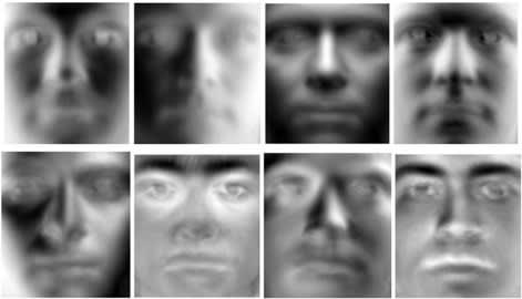
This is pretty cool! We’re basically getting versions of the “general shape of a human face”. The first few capture broad patterns of shading & basic features, while the later ones capture features such as lips, eyes and shadows in more detail.

If we wanted to compress a face image into a small number of dimensions and transmit it, we might find the projections of our face along the first few “eigenfaces”. To make this more concrete, for an image $\text{x}$ of shape (width, height), we might flatten this into a vector of length $m$, then calculate the $k$-dimensional vector $\widehat{U^T}\text{x}$ (which is equivalent to finding the projections of $x$ along the first $k$ columns of $U$), and then reconstruct by multiplying by $\hat{U}$.

If we wanted to generate a completely new face from scratch, we could choose a feature vector (i.e. some unit vector in $n$-dimensional space), and then map it through $\hat{M}=\hat{U}\hat{S}\widehat{V^T}$. This would give you a face which has “exposure to the $i$-th eigenface” equal to the $i$-th element of your chosen feature vector.

Final Thoughts

Recapping these, we find that the SVD:

1. Is a decomposition of complicated linear operations into simpler components (rotations and scalings),

2. Allows us to best approximate a matrix with one of smaller rank,

3. Is the natural way to express solutions to least-squares type equations,

4. Gives us a set of independent input and output directions which fully describe the linear transformation,

5. Tells us what information gets lost and what gets preserved by the linear transformation,

6. Has a natural interpretation when our matrix is a data matrix (for example, when each datapoint is a flattened image—eigenfaces!).

Appendix—First-Principles Proof of SVD

First, a quick rant. It bugs me how almost all the proofs of SVD use the spectral theorem or some variant. This seems like massive overkill to me, when there’s actually a very elegant proof which just uses some basic calculus, and also gets to the essence of SVD in a way that the spectral theorem-based proofs just don’t. For that reason, I’m including this proof in the post.

Sketch of proof

Our proof involves choosing $({\sigma }_i,{\text{u}}_i,{\text{v}}_i)$ sequentially, until we’ve spanned all of $M$. At each step, we find unit vector ${\text{v}}_i$ to maximize $\parallel M{\text{v}}_i\parallel$, subject to ${\text{v}}_i$ being orthogonal to our previously chosen vectors. Then we define ${\sigma }_i=\parallel M{\text{v}}_i\parallel$ and ${\text{u}}_i=\frac{1}{{\sigma }_i}M{\text{v}}_i$. The only non-trivial part of our proof will be showing that ${\text{u}}_i$ are orthogonal to each other. This will involve a short geometric argument.

Actual proof

We’ll sequentially choose $({\sigma }_i,{\text{u}}_i,{\text{v}}_i)$, using the following algorithm:

• We define ${\text{v}}_i=\underset{\parallel \text{v}\parallel =1}{\max }\parallel M\text{v}\parallel$ subject to the restriction ${\text{v}}_i\perp {\text{v}}_j$ for all $j<i$

• We define ${\sigma }_i=\parallel M{\text{v}}_i\parallel$ and ${\text{u}}_i=\frac{1}{{\sigma }_i}M{\text{v}}_i$.

Most of the properties of SVD are already proved from this algorithm. By our definition, ${\text{v}}_i$ are orthogonal unit vectors, ${\text{u}}_i$ are unit vectors, and ${\sigma }_i$ are strictly positive & non-increasing (because each ${\text{v}}_i$ is chosen with more restrictions than the previous one). The algorithm terminates when $M{\text{v}}_i=0$ for all possible choices of ${\text{v}}_i$, at which point the $\text{v}$-vectors we’ve chosen so far must span the domain of $M$, and we’re done. The only thing left is to show that the $\text{u}$-vectors are orthogonal.

Suppose $j<i$, and so ${\sigma }_j>{\sigma }_i>0$. We can define the function $f\left(\theta \right)=\parallel M{\text{v}}_j\cos \theta +M{\text{v}}_i\sin \theta {\parallel }^2$. We know that ${\text{v}}_j$ was chosen to maximise $\parallel M{\text{v}}_j\parallel$ subject to orthogonality with the other $v$-vectors, which means (since $v_i$ is also orthogonal to the other $v$-vectors) that $\theta =0$ must be a stationary point of the function $f$. But if we Taylor-expand $f\left(\theta \right)$ around $\theta =0$, we get:

$$f\left(\theta \right)=\parallel M{\text{v}}_j\cos \theta +M{\text{v}}_i\sin \theta {\parallel }^2=\parallel M{\text{v}}_j{\parallel }^2+2\left(M{\text{v}}_i{)}^T\right(M{\text{v}}_j)\theta +O({\theta }^2)$$

and so $f^{\prime }\left(0\right)=0$ implies $\left(M{\text{v}}_i{)}^T\right(M{\text{v}}_j)=0$, hence ${\text{u}}_i^T{\text{u}}_j=0$, as required.

The image below shows the geometric intuition for this proof. If $M{\text{v}}_i$ and $M{\text{v}}_j$ weren’t orthogonal, then we’d be able to define ${\text{v}}_j^{\prime }$ by rotating ${\text{v}}_j$ a small amount wrt ${\text{v}}_i$, and this would result in a larger vector $M{\text{v}}_j$ (contradiction, since ${\text{v}}_j$ was chosen to maximise $M{\text{v}}_j$).

Appendix—Eckart-Young Theorem

Firstly, let’s prove the two lemmas.

The squared Frobenius norm of a matrix equals the sum of its squared singular values.

Sketch of proof—left-multiplying $M$ by an orthogonal matrix is equivalent to doing a unitary operation on the columns of $M$. Since the squared Frobenius norm is the sum of squared $L_2$ norms of columns, and unitary operations don’t change the $L_2$ norm, $M$ and $U^{T}M=S{V}^T$ must have the same Frobenius norm. A similar argument (rows rather than cols) shows that we can right-multiply by an orthogonal matrix without changing the Frobenius norm. So $M$ and $U^{T}MV=S$ have the same Frobenius norm. But $S$ is a diagonal matrix elements equal to the singular values, so $\parallel S{\parallel }_F^2$ is clearly the sum of squared singular values.

The spectral norm of a matrix is its largest singular value.

This follows directly from the way we proved the SVD—we chose ${\text{v}}_1$ to maximize $\parallel M\text{v}\parallel$ over all possible vectors $\text{v}$ of unit norm.

Now, let’s prove the full theorem. Both spectral and Frobenius norm are unchanged by unitary operations, so we have $\parallel M-M_k\parallel =\parallel S-A_k\parallel$ for both types of norm (where $A_k=U^T{M}_{k}V$ has the same rank as $M_k$). If we choose $A_k=S_k$ (the diagonal matrix formed from the first $k$ singular values of $S$), then we get $\parallel S-A_k{\parallel }_2={\sigma }_{k+1}$, and $\parallel S-A_k{\parallel }_F^2={\sum }_{i=k+1}^r{\sigma }_i^2$. It remains to prove that we can’t do better than this.

For a general rank-$k$ matrix $A_k$, we can find a vector $\text{f}$ in the span of the standard basis vectors $({\text{e}}_1,{\text{e}}_2,...,{\text{e}}_{k+1})$ s.t.$\text{f}$ is in the nullspace of $A_k$. Then we have:

$$\parallel S-A_k{\parallel }_2\ge \parallel (S-A_k)\text{f}{\parallel }_2=\parallel S\text{f}\parallel \ge \parallel {\sigma }_{k+1}\text{f}\parallel ={\sigma }_{k+1}$$

proving the result for spectral norm. Similarly, we can find vectors ${\text{f}}_{k+1},...,{\text{f}}_r$ in the span of $({\text{e}}_1,{\text{e}}_2,...,{\text{e}}_r)$ which are all in the nullspace of $A_k$. Using the invariance of the Frobenius norm to changes in basis, we have:

$$\parallel S-A_k{\parallel }_F^2\ge \sum _{i,j=k+1}^r\left({\text{f}}_i^T\right(S-A_k){\text{f}}_j{)}^2=\sum _{i,j=k+1}^r({\text{f}}_i^{T}S{\text{f}}_j{)}^2=\sum _{i=k+1}^r{\sigma }_i^2$$

so we’re done.

1. ^

   Citation needed.

2. ^

   Note, the Eckart-Young Theorem is sometimes used to refer to the Frobenius norm, sometimes to the spectral norm, and sometimes to both.

3. ^

   For more on this, see Evan Chen’s Napkin Linear Algebra section, or his rant on why matrices are not arrays of numbers.

4. ^

   Note that this terminology is not standard (as far as I know).

5. ^

   The proof is left as an exercise to the reader. Hint—start by writing the Lagrangian $L(x,\lambda )=\parallel Mx-b{\parallel }_2^2+\lambda (m^2-\parallel x{\parallel }_2^2)$.

6. ^

   There’s a similar story if we had the constraint $\parallel x{\parallel }_1\le m$. Our solution here is found by trying to set $x_{v_i}=b_{u_i}/{\sigma }_i$ for as many $i=1,2,...$ as possible, until we hit our constraint. In other words, we only care about matching the components of $x$ along the most important input directions (unlike the $L_2$-restricted case, where we just weighted the more important input directions more highly than the less important ones).

7. ^

   That is, if we’re quantifying “best” by the norm of the approximation residual, for a choice of norm like Frobenius or $L_2$ (see the section on least squares).

8. ^

   They’re eigenvectors of the matrix $M{M}^T=U{S}^2{U}^T$.

[Joseph Van Name]

The singular value decomposition is great and it even works well for complex and quaternionic matrices (and we can even generalize decompositions like the spectral, polar, and singular value decomposition and apply them to bounded linear operators between infinite dimensional Hilbert spaces), but to get a better appreciation of the singular value decomposition, we ought to analyze its deficiencies as well. I am currently researching other linear dimensionality reduction techniques (namely LSRDRs) that work well in the cases when the singular value decomposition is not the best technique to use for a linear dimensionality reduction. These cases include the following:

1. While the SVD approximates a matrix with a low rank matrix, it does not generalize that well to higher order SVDs that decompose tensors in $V_1\otimes V_2\otimes \cdots \otimes V_n$ where $V_1,\dots ,V_n$ are vector spaces.

2. The SVD works applies to linear mappings between inner product spaces, but the SVD does not take any additional structure that the linear mappings or inner product spaces have. For example, if we had a tuple of vectors $(v_1,\dots ,v_r)$, then we may want to use a linear dimensionality reduction that does not just consider $(v_1,\dots ,v_r)$ as a matrix. For example, it is more meaningful to consider a weight matrix in a neural network as a tuple of row vectors or a tuple of column vectors than just a matrix without additional structure.

3. If we apply the principal component analysis to a collection $(v_1,\dots ,v_r)$ of vectors (with mean 0 for simplicity), then the $k$-dimensional subspace $M$ that best approximates $(v_1,\dots ,v_r)$ may fail to cluster together. For example, suppose that $X_1,\dots ,X_s,Y_1,\dots ,Y_s$ are independent normally distributed random variables each with mean 0 where each $X_j$ has covariance matrix $I_n\oplus 0.1\cdot I_n$ while each $Y_j$ has covariance matrix $0.1\cdot I_n\oplus I_n$. If we take a random sample $(x_1,\dots ,x_s,y_1,\dots ,y_s)$ from $X_1,\dots ,X_s,Y_1,\dots ,Y_s$ and then perform a principal component analysis to $(x_1,\dots ,x_s,y_1,\dots ,y_s)$ to find an $n$-dimensional subspace of $R^n\oplus R^n$, then the principal component analysis will not tell you anything meaningful. We would ideally want to use something similar to the principal component analysis but which instead returns subspaces that are near $R^n\oplus \left\{0\right\}$ or $\left\{0\right\}\oplus R^n$. The principal component analysis returns the top $k$-dimensional affine subspace of a vector space in magnitude, but the principal component analysis does not care if the canonical basis for these $k$-dimensions form a cluster in any way.

4. Every real, complex, or quaternionic matrix has an SVD, and the SVD is unique (except in the case where we have repeated singular values). While mathematicians tend to like it when something exists and is unique, and computer scientists may find the existence and uniqueness of the singular value decomposition to be useful, the existence and uniqueness of the SVD does have its weaknesses (and existence and uniqueness theorems imply a sort of simplicity that is not the best indicator of good mathematics; good mathematics is often more complicated than what you would get from a simple existence and uniqueness result). One should consider the SVD as a computer program, programming language, and piece of code that always return an output regardless of whether the output makes sense without ever producing an error message. This makes it more difficult to diagnose a problem or determine whether one is using the correct tools in the first place, and this applies to the singular value decomposition as well. The poor behavior of an algorithm could also provide some useful information. For example, suppose that one is analyzing a block cipher round function $E$ using an algorithm $L$. If the algorithm $L$ produces errors for complicated block cipher round functions but does not produce these errors for simple block cipher round functions, then the presence of one or more errors indicates that the block cipher round function $E$ is secure.

5. If $A$ is a real matrix, but we take the complex or quaternionic SVD of $A$ to get a factorization $A=UD{V}^{\ast }$, then the matrices $U,V$ will be real orthogonal matrices instead of complex or quaternionic matrices. This means that the SVD of a matrix is always well-behaved which is again a problem since this well-behavedness does not necessarily mean that the singular value decomposition is useful for whatever circumstances we are using it for and the poor behavior of a process may provide useful information.

6. The SVD is not exactly new or cutting edge, so it will give one only a limited amount of information about matrices or other objects.

Let $K$ denote either the field of real numbers, the field complex numbers, or the division ring of quaternions. Suppose that $A_1,\dots ,A_r$ are $n\times n$-matrices with entries in $K$. If $X_1,\dots ,X_r$ are $d\times d$-matrices, then define an superoperator $\Gamma (A_1,\dots ,A_r;X_1,\dots ,X_r):M_{n,d}\left(K\right)\to M_{n,d}\left(K\right)$ by letting $\Gamma (A_1,\dots ,A_r;X_1,\dots ,X_r)\left(X\right)=A_{1}X{X}_1^{\ast }+\cdots +A_{r}X{X}_r^{\ast }$ whenever $X\in M_{n,d}\left(K\right)$. Define a partial (but nearly total) function $F_{A_1,\dots ,A_r;K}:M_d(K{)}^r\to [0,\infty )$ by letting

$F_{A_1,\dots ,A_r;K}(X_1,\dots ,X_r)=\frac{\rho \left(\Gamma \right(A_1,\dots ,A_r;X_1,\dots ,X_r\left)\right)}{\rho \left(\Phi \right(X_1,\dots ,X_r){)}^{1/2}}$. Here, let $\rho$ denote the spectral radius of a linear operator. We say that $(X_1,\dots ,X_r)$ is a $L_{2,d}$-spectral radius dimensionality reduction (LSRDR) of type $K$ if the quantity$F_{A_1,\dots ,A_r;K}(X_1,\dots ,X_r)$ is locally maximized.

One can compute LSRDRs using a flavor of gradient ascent. Don’t worry. Taking an approximate gradient of the $F_{A_1,\dots ,A_r;K}$ is less computationally costly than it sounds, and the gradient ascent should converge to an LSRDR $(X_1,\dots ,X_r)$. If the gradient ascent process fails to quickly converge to an LSRDR $(X_1,\dots ,X_r)$, then LSRDRs may not be the best tool to use.

We say that $(X_1,\dots ,X_r),(Y_1,\dots ,Y_r)$ are projectively similar and write $(X_1,\dots ,X_r){\simeq }_K(Y_1,\dots ,Y_r)$ if there is some $\alpha \in Z\left(K\right)$ ($Z\left(K\right)$ denotes the center of $K$) and some invertible matrix $R$ such that $X_j=\alpha R{Y}_j{R}^{-1}$ for $1\le j\le r$. Let $[X_1,\dots ,X_r{]}_K$ denote the equivalence class containing $(X_1,\dots ,X_r)$.

The equivalence class $[X_1,\dots ,X_r{]}_K$ of an LSRDR of type $K$ of $(A_1,\dots ,A_r)$ is often unique. At the very least, one should only be able to find a few equivalence classes $[X_1,\dots ,X_r{]}_K$ of LSRDRS of type $K$ of $(A_1,\dots ,A_r)$, and the equivalence class $[X_1,\dots ,X_r{]}_K$ of LSRDRs with highest fitness should also be the easiest to find. But if the equivalence class $[X_1,\dots ,X_r{]}_K$ is far from being unique, then this should be an indicator that the notion of taking an LSRDR may not be the best tool to use for analyzing $(A_1,\dots ,A_r)$, so one should try something else in this case.

If $A_1,\dots ,A_r$ are all real matrices but $K=C$, then the equivalence class $[X_1,\dots ,X_r{]}_K$ of the LSRDR should contain a tuple $(Y_1,\dots ,Y_r)$ where each $Y_i$ is a real matrix. One can quickly test whether one should be able to find such a tuple $(Y_1,\dots ,Y_r)$ given an LSRDR $(X_1,\dots ,X_r)$ is to compute $\frac{\text{Tr}\left(X_i\right)}{\text{Tr}\left(X_j\right)}$. If $\frac{\text{Tr}\left(X_i\right)}{\text{Tr}\left(X_j\right)}$ is a real number (up-to a rounding error), then that means that the LSRDR is well-behaved and perhaps an appropriate tool to use, but otherwise the LSRDR may not be the best tool to use.

If we find our LSRDR $(X_1,\dots ,X_r)$ of type $K$ of $(A_1,\dots ,A_r)$, then if everything works out well, there should be some matrices $R,S$ where $X_j=R{A}_{j}S$ for $1\le j\le s$ and where $RS=\lambda \cdot 1_d$ and where $SR=\lambda \cdot P$ for some (not necessarily orthogonal) projection matrix $P$ and constant $\lambda \in Z\left(K\right)$. If $\lambda =1$, then we say that $R,S$ is constant factor normalized; if $R,S$ is constant factor normalized, then $RS=1_d,SR=P$, so let us assume that $R,S$ is constant factor normalized to make everything simpler. Let $U_R$ be the dominant eigenvector of $\Gamma (A_1,\dots ,A_r;X_1,\dots ,X_r)$, and let $U_L$ be the dominant eigenvector of $\Gamma (A_1,\dots ,A_r;X_1,\dots ,X_r)$. Then there are positive semidefinite matrices $G,H$ and non-zero constants ${\mu }_G,{\mu }_H\in Z\left(K\right)$ where$U_R{S}^{\ast }={\mu }_H\cdot H,U_{L}R={\mu }_G\cdot G$. The projection matrix $P$ should be recovered from the positive semidefinite matrices $G,H$ since $\text{Im}\left(H\right)=\text{Im}\left(P\right),\text{Im}\left(G\right)=\ker (P{)}^{\perp }$, and the positive semidefinite matrices $G,H$ (up-to a constant real factor) should be uniquely determined. The positive semidefinite matrices $G,H$ should be considered to be the dominant clusters of dimensions for $(A_1,\dots ,A_r)$.

Order 2 tensors: Suppose that $v_1,\dots ,v_r\in V$ for some finite dimensional real inner product space $V$. Then set $A_j=v_j{v}_j^{\ast }$ for $1\le j\le r$. Then $G=H$, so the positive semidefinite matrix $G$ is our desired dimensionality reduction of $v_1,\dots ,v_r$. For example, if $M$ is a weight matrix in a neural network, then we can make $v_1,\dots ,v_r$ the columns of $M$, or we can make $v_1,\dots ,v_r$ the transposes of the rows of $M$. Since we apply activation functions before and after we apply $M$, it makes sense to separate $M$ into rows and columns this way. And yes, I have performed computer experiments that indicate that for $A_j=v_j{v}_j^{\ast }$, the matrices $G,H$ do represent a cluster of dimensions (at least sometimes) rather than simply the top $d$ dimensions. I have done the experiment where $(v_1,\dots ,v_r)=(x_1,\dots ,x_s,y_1,\dots ,y_s)$ and in this experiment, the matrices $G,H,P$ (up to a constant factor for $G,H$) are all approximately the projection matrix that projects onto the subspace $R^n\oplus \left\{0\right\}$.

Order 3 tensors: Suppose that $V,W$ are finite dimensional real or complex inner product spaces and $A:V\to V\otimes W$ is a linear mapping. Observe that $L(V,V\otimes W)$ is canonically isomorphic to $V\otimes V\otimes W$. Now give $W$ an orthonormal basis $e_1,\dots ,e_r$, and set $A_j=(1_V\otimes e_j^{\ast })A$ for $1\le j\le r$. Then one can apply an LSRDR to $A_1,\dots ,A_r$ to obtain the positive semidefinite matrices $G,H$. The positive semidefinite matrices $G,H$ do not depend on the orthonormal basis $e_1,\dots ,e_r$ that we choose. For example, suppose that $O_1,O_2$ are open subsets of Euclidean spaces of possibly different dimensions and $f:O_1\to O_2$ is a $C^2$-function where there are $f_1,\dots ,f_r:O_1\to R$ where $f\left(x\right)=\left(f_1\right(x),\dots ,f_r(x\left)\right)$ for each $x\in O_1$. Then let $A_j=H\left(f_j\right)\left(x\right)$ for $1\le j\le r$ where $H\left(f_j\right)$ denotes the Hessian of $f_j$. Then the matrices $G,H$ of an LSRDR of $A_1,\dots ,A_r$ represent a cluster of dimensions in the tangent space at the point $x$.

Order 4 tensors: Given a vector space $V$, let $L\left(V\right)$ denote the collection of linear maps from $V$ to $V$. Let $V$ be a finite dimensional complex inner product space. Then there are various ways to put $V\otimes V\otimes V\otimes V$ into a canonical one-to-one correspondence with $L\left(L\right(V\left)\right)$. Furthermore, the Choi representation gives a one-to-one correspondence between the completely positive operators in $L\left(L\right(V\left)\right)$ and the positive semidefinite operators in $L(V\otimes V)$. An operator $E\in L\left(L\right(V\left)\right)$ is completely positive if and only if there are $A_1,\dots ,A_r\in L\left(V\right)$ where $E\left(X\right)=A_{1}X{A}_1^{\ast }+\cdots +A_{r}X{A}_r^{\ast }$ for all $X\in L\left(V\right)$. Therefore, whenever $E$ is completely positive, we compute a complex LSRDR $(X_1,\dots ,X_r)$ of $(A_1,\dots ,A_r)$, and we should get matrices $R,S,P,G,H$, and $G,H$ give us our desired dimensionality reduction. Of course, given an order 4 tensor, one has to ask whether it is appropriate to use LSRDRs for this order 4 tensor, and one should ask about the best way to use these order 4 tensors to produce an LSRDR.

If this comment were not long enough already, I would give an explanation for why I believe LSRDRs often behave well, but this post is really about the SVDs so I will save my math for another time.