Automatically finding feature vectors in the OV circuits of Transformers without using probing

[Jacob Dunefsky]

Let’s say that you’re working to understand how a given large language model computes its output on a certain task. You might be curious about the following questions:

• What are some linear feature vectors that are responsible for the model’s performance on a given task?

• Given a set of different tasks, to what extent are the same features responsible for the model’s outputs on these different tasks?

• How do nonlinearities such as LayerNorm transform the features that are used for a given task?

• Given a pair of features, if the value of one feature for an input is high, then does this imply that the value of another feature for that input is likely to be high?

• How can I find a steering vector to add to the activations of a model that increase the model’s output on one task while decreasing its output on another?

Recently, I’ve been working on developing a general method that yields partial answers to these questions. Notably, unlike probing methods for finding feature vectors, this method can find approximate answers to these questions with zero forward passes on data, yielding improved answers with very few additional datapoints^[1]. This post introduces this method for finding feature vectors, dubbed “observable propagation”; puts forth theoretical results regarding the analysis of feature vectors yielded by observable propagation; and presents the results of some preliminary experiments testing this method.

Note that this is all very much a work in progress! There are many more experiments that I am currently running, in order to obtain a better understanding of the utility and limits of observable propagation. Additionally, I still have to clean up my code before making it public (although the methods described here shouldn’t be too hard to re-implement). But rather than wait for everything to be finished before sharing the results that I do have, I figured that it would be best to present the work that I’ve completed thus far to the community.

The contributions of this work are as follows:

• This work introduces the concept of “observables” that generalizes the pattern of considering a model’s performance on a task by looking at logit differences. A number of new techniques for analyzing Transformers opens up once one starts treating observables as concrete objects amenable to study.

• This work presents a method called “observable propagation” that allows one to find feature vectors in the OV circuit of a Transformer corresponding to any given observable. Note that this method can find feature directions, along with approximate feature magnitudes, without requiring any additional data. This method can be extended to nonlinear components in Transformers using small amounts of data in order to obtain better approximations of feature magnitudes.

• This work develops a theory for the analysis of feature vectors. This includes a theorem that LayerNorm nonlinearities do not affect feature directions in high-dimensional space (although they do affect feature magnitudes). This work also introduces a similarity metric called the “coupling coefficient”, which measures the expected dot product between an input and a feature vector given that the input’s dot product with another feature vector is equal to 1.

• I apply observable propagation to the problem of gendered pronoun prediction considered in by Chris Mathwin et al. as a case study. I extend their problem setting by considering the case of both object and subject pronoun prediction, and demonstrate that in both cases, many of the same features are being used. I also find that looking at the norms of feature vectors associated with different attention heads provides a good initial prediction of which attention heads end up contributing the most to the output. I show that some feature vectors found by observable propagation do not cleanly align with the singular vectors of their respective attention heads, indicating that observable propagation can find feature vectors that SVD might miss.

• Finally, I demonstrate some preliminary results on using these feature vectors as activation steering vectors in order to reduce the amount of gender bias displayed by the model.

Epistemic status: I am very confident that observable propagation, along with the theory of LayerNorms and coupling coefficients, accurately describes the OV circuits of non-MLP Transformers, and can make accurate predictions about the behavior of these OV circuits. I am also somewhat confident that feature vector norms can be used to make decent “educated guesses” regarding the attention heads important for a task, although I’d have to perform more experiments on more tasks in order to become more certain one way or the other. I am still uncertain, however, about the extent to which understanding QK behavior is necessary for understanding Transformers. I am also still in the process of determining the extent to which these methods can be applied to MLPs. Regarding the experiments presented here: the work on the pronoun prediction task is more developed than the work on the gender bias task, which is currently more in the exploratory stage.

TL;DR

If we have a task that we would like to evaluate our model on—for instance, the logit difference between token A and token B—then we can construct a linear functional corresponding to that task. (For example, the logit difference between token A and token B corresponds to the linear functional $n^T=(e_A-e_B{)}^T$, where $e_A$ is the one-hot vector with a 1 in the position corresponding to token A.) I refer to linear functionals on the logits as observables, inspired by the concept from quantum mechanics.

Once we have an observable $n^T$, then given an attention head $h$, the feature vector for that attention head corresponding to the observable $n^T$ is given by ${\left(W_h^{OV}\right)}^{T}n$, where $W_h^{OV}$ is the OV matrix for attention head $h$. This can be extended to virtual attention heads simply by multiplying their OV matrices, and can be extended to deal with nonlinearities by taking their linear approximations. I prove that in high dimensions, LayerNorms do not change feature vector directions—although LayerNorms do affect feature vector magnitudes. I refer to this general method for finding feature vectors given observables as “observable propagation”.

After observable propagation yields feature vectors, we can then analyze them without running the model on any data. For instance, we can look at feature vector norms to get an initial prediction of which attention heads are likely to be important. We can also compare feature vectors for two different observables by looking at their cosine similarities; this allows us to understand when two circuits for different tasks use the same features. I also define the “coupling coefficient” from feature vector $v_1$ to feature vector $v_2$ as $\frac{v_1\cdot v_2}{\parallel v_1{\parallel }^2}$, and prove that this represents the expected dot product between a normally-distributed embedding vector $x$ and feature vector $v_2$ given that $x\cdot v_1=1$.

I performed some initial experiments applying observable propagation to the setting of gendered pronoun prediction. Preliminary results suggest that feature vector norms do generally correspond with active attention heads; that subject pronoun prediction and object pronoun prediction use the same feature vectors; and that the feature vectors yielded by observable propagation can be used as activation steering vectors to successfully change the model’s output.

Introduction: meet observables

When we want to understand how a model performs on a task, it’s very common to look at a “logit difference” that corresponds to that task. For instance, when Joseph Miller and Clement Neo look into what causes a model to predict the token ” an” instead of ” a”, they perform activation patching with respect to the difference between the model’s predicted logits for ” an” and ” a”. Similarly, in gendered pronoun prediction, Chris Mathwin et al. consider the logit difference between ” he” and ” she”. Taking logit differences is recognized as an important part of the interpretability workflow: Neel Nanda explains it as “a really good metric to judge model performance with various interpretability-inspired interventions and techniques (eg direct logit attribution or activation patching)”.

But our first insight here is to go beyond treating logit differences as a mere step in an experimental process. Instead, we want to treat them as concrete objects that can be studied and manipulated mathematically. What sort of object? Well, if we take the logit difference between token $a$ and token $b$, then what we are really doing is calculating $(e_a-e_b{)}^{T}v$ where $v$ is the vector of logits and $e_x$ is the one-hot vector with a one in position $x$. The object $(e_a-e_b{)}^T$ is a linear functional: a linear map from a vector space to the real numbers. Clearly, all logit differences are linear functionals on the logits. And it turns out that there are linear functionals that we might want to consider beyond simply logit differences between two tokens. For example, we might consider the linear functional $(e_{\text{" she"}}+e_{\text{" her"}}-e_{\text{" he"}}-e_{\text{" him"}}{)}^T$ to represent the task of predicting of female gendered pronouns in general.

Motivated by this, we have the following definition: an observable is a linear functional on the logits^[2][3]. The idea is that a large class of tasks that we might care about evaluating can be formalized as linear functionals on the logits. And once we have done so, we can then apply the tools of linear algebra to find feature vectors corresponding to observables.

Finding feature vectors via observable propagation

Now, I’ll present a process for finding feature vectors corresponding to observables. I call this method “observable propagation”, because it involves propagating observables backward through the network. In this section, we’ll start by understanding observable propagation in simpler cases, and then build up to greater generality.

Basic linear models

The basic insight behind observable propagation is very simple. Say that we have a linear model: $f\left(x\right)=Wx$ for some matrix $W$. Given an observable $n$, we want to find some feature vector $y$ corresponding to this observable. This means that we want to find $y$ such that $y\cdot x=n\cdot f\left(x\right)$. Now watch: $n\cdot f\left(x\right)=n^{T}Wx=(W^{T}n{)}^{T}x=(W^{T}n)\cdot x$. Therefore, $y=W^{T}n$. In one line of simple linear algebra, we have precisely found the feature vector corresponding to $n$.

Note that this also works in the affine case, where $f\left(x\right)=Wx+b$ for some $b$. In this case, we have that $n\cdot f\left(x\right)=(y\cdot x)+c$ for a scalar constant $c$ -- but this still means that $y$ is the direction in embedding space that “directly determines” the output $n\cdot f\left(x\right)$.

Aside: differences between observable propagation and related methods

This result is very clean, and yet, to my knowledge, no one else has yet made use of it. This was very surprising to me! A few other works have touched upon similar ideas, though, and I found it worthwhile to consider where my formulation diverges from theirs.

In “We found an neuron in GPT-2″, Joseph Miller and Clement Neo attempt to find neurons in GPT-2 that are responsible for predicting certain tokens (with a particular focus on the token ” an”). They do so, in part, by taking the dot product of the token embedding with each neuron output weight (i.e. each column of the weight matrix) and looking at the neurons with the highest dot products. If we store the results of this process in a vector $y$, then we have $y=W^{T}n$ where $n$ is a one-hot vector with a one in the position for the token that we care about, and $W$ is the output weight matrix. However, the authors don’t make this conceptual leap towards considering $y$ as a feature vector, rather than just a list of dot products. Instead, the authors seem to operate under the paradigm in which the goal is to interpret neurons, or groups of neurons, rather than more general feature vectors. This approach can yield some success—but it doesn’t account for non-basis-aligned features, or more complex concepts such as superposition.

In “The Singular Value Decompositions of Transformer Weight Matrices are Highly Interpretable”, Beren Millridge and Sid Black show that the singular vectors of Transformer weight matrices yield interpretable sets of tokens when projected into token space using the model’s unembedding matrix. They then demonstrate that you can find singular vectors corresponding to specific tokens by first finding those tokens’ embeddings, and then looking at the cosine similarity between the tokens’ embeddings and the singular vectors; the singular vectors with the highest cosine similarity are then considered the most likely to correspond to the given tokens. But note that their work primarily looks to choose from among a set of singular vectors the one with the highest relevance for a given token, even if none of the singular vectors align well with that token. As such, their framing is the same as in “We found an neuron in GPT-2″: instead of considering general feature vectors, they first consider a set of feature vectors, and then choose the feature vector from that set that is the most relevant to a given “query”. Additionally, their work only looks at singular vectors corresponding to tokens, rather than those corresponding to more general observables.

Thus, as I see it, there are two generalizations that the “observable propagation” method makes, that aren’t made in the above two works:

• The feature vectors that we care about might not be found among a small set of basis vectors (e.g. neurons or singular vectors).

• We want to go beyond finding feature vectors associated with specific tokens, and instead consider feature vectors associated with more general tasks. (In the “observable propagation” formulation, these “more general tasks” correspond to linear functionals on the logits.)

I believe that it’s these generalizations that have to be internalized before you view the equality $n\cdot Wx=\left(W^{T}n\right)\cdot x$ as something meaningful for interpretability. This, of course, raises the following question: what generalizations am I missing now? We’ll come back to this question later.

Also, while the aforementioned works of research are the ones that I found to be most relevant to the method of observable propagation, it’s always possible that I missed an article or post in my literature review. If that’s the case, please let me know.

Interpreting OV circuits

Single attention heads

We now have a means of going from any observable to any feature vector, if the model that we’re considering is linear. Unfortunately, even an attention-only Transformer is nonlinear. To begin with, the process of computing attention scores involves a bilinear operation on multiple tokens followed by a softmax. And then, a linear function of each token is then multiplied by these attention scores.

However, this problem can be mitigated by only looking at what the original Transformer Circuits formulation calls the “OV circuit” of attention. The idea is that attention can be decomposed into two “circuits”: a computation that determines from which tokens information is read, and a computation what information is written from those tokens. The former computation is called the “QK circuit”, and the latter computation is called the “OV circuit”. Now, if we treat attention scores as fixed constants, then what we’re doing is ignoring the nonlinear QK circuit, and instead, looking only at the OV circuit—which is an affine function of all the tokens. Indeed, recall that an attention layer in a Transformer can be decomposed as

$$x_j^{l+1}=x_j^l+\sum _{\text{attention head}h}\sum _{\text{token index}i}{\mathrm{score}}_h(x_i^l,x_j^l)W_{l,h}^{OV}{x}_i^l$$

where $x_j^l$ is the residual stream for token $j$ at layer $l$, ${\mathrm{score}}_{l,h}(x_i^l,x_j^l)$ is the attention score at layer $l$ associated with attention head $h$ for tokens $x_i^l$ and $x_j^l$, and $W_{l,h}^{OV}$ is the combined output-value weight matrix for attention head $h$ at layer $l$. As such, given an observable $n$, we have that the feature vector for attention head $h$ at layer $l$ is given by

$$y_{l,h}=(W_{l,h}^{OV}{W}_U{)}^{T}n$$

where $W_{l,h}^{OV}$ is the combined output-value weight matrix for attention head $h$ at layer $l$, and $W_U$ is the token unembedding matrix. Note that this works for attention heads at any layer, because all attention heads’ contributions at each layer stick around in the residual stream of the Transformer (and even if these contributions are later overwritten, they were still output into the residual stream in the first place).

Virtual attention heads

The next step at this point is to note that the output of one attention head can be used as the input to another attention head. The result is called a “virtual attention head” in the Transformer Circuits formulation. Finding feature vectors for virtual attention heads is simple: given attention heads $h,h^{\prime }$ at layers $l,l^{\prime }$ respectively with $l<l^{\prime }$, the feature vector associated with head $h$ at layer $l$, as mediated through head $h^{\prime }$ at layer $l^{\prime }$, is given by

$$y_{l,h}=(W_{l,h}^{OV}{W}_{l^{\prime },h^{\prime }}^{OV}{W}_U{)}^{T}n.$$

Of course, this works for attention head composition of arbitrary length—simply multiply out all relevant heads’ $W^{OV}$ matrices.

Looking at virtual attention heads is a very important step in interpreting a Transformer’s computation: if you only look at the direct contribution that attention heads have on the output logits, then you’ll end up missing information crucial to understanding what’s actually happening under the hood. We’ll later discuss a case in which it initially seemed that the model used very different feature vectors to compute its output corresponding to two different observables—but when we looked at virtual attention heads, we found that these models were actually using the same feature.

Is it okay to ignore the QK circuit?

Recall that all of this analysis only looks at OV circuits; it doesn’t consider at all the feature directions that affect the model by changing which tokens it reads information from. We should therefore ask ourselves: is this reasonable? To what extent can we say that these feature vectors capture the behavior of the model, when they don’t take into account an integral part of the attention computation?

As we’ll later see when we discuss experimental results, even if observable propagation does yield an incomplete description of the model because of this, it still boasts some real utility: it gives good zero-shot predictions of attention heads relevant to a given task, it gives us zero-shot steering vectors that can be used to alter the model’s behavior, it gives us a good understanding of the degree to which one attention head’s output is correlated with another. My take is that OV circuits do account for a large amount of the model’s behavior in many tasks that we’re interested in (e.g. the tasks discussed in this article), and that for at least those tasks, observable propagation can be a very good way to understand model behavior.

Dealing with nonlinearities

Alas! Transformers used in the real world are not attention-only. The two types of per-token nonlinearities in Transformers are LayerNorms and MLPs. Our solution for dealing with them is simple: just take their linear approximation using their gradient. More specifically, if we have some nonlinear function $f:R^d\to R^d$, then for a given observable $n$, we approximate $g\left(x\right)=n\cdot f\left(x\right)$ at $x_0$ as $n\cdot f\left(x_0\right)+(x-x_0)\cdot \nabla g\left(x_0\right)$. As we can see, $n\cdot f\left(x\right)$ is approximately equal to $\nabla g\left(x_0\right)\cdot x$ plus some additive constant. Therefore, the feature vector associated with $f$ for observable $n$ is $g\left(x_0\right)$.

Of course, care must be taken to choose a good point $x_0$ at which we approximate $f$. What I found to be sensible was to take an embedding $x_{-}$ from the dataset being used such that $n\cdot f\left(x_{-}\right)<0$, and an embedding $x_{+}$ such that $n\cdot f\left(x_{+}\right)>0$. Then, you chose $x_0$ to be a point on the line between $x_{-}$ and $x_{+}$ such that $n\cdot f\left(x_0\right)=0$. The idea is that the gradient at the decision boundary of $n\cdot f\left(x\right)$ should capture the larger-scale behavior of the nonlinear $f$ that causes $n\cdot f\left(x\right)$ to be positive or negative; if we took the gradient at $x_{-}$ or $x_{+}$, then the nonlinearity might already be saturated, and therefore, the nonlinearity’s behavior there might not be indicative of its broader behavior.

Now, if we have a computational path that involves going through a nonlinearity (e.g. an attention head followed by a LayerNorm followed by another attention head), then given an observable $n$ we can compute the overall feature vector as follows. First, compute the feature vector for $n$ associated with the nonlinearity; call this feature vector $y_1$. Then, treat this feature vector as the new observable, and compute the feature vector for the lower-layer component with respect to the “observable” $y_2$. Rinse and repeat as necessary^[4].

Here, it’s worth mentioning “attribution patching”, work done by Neel Nanda, Chris Olah, Catherine Olsson, Nelson Elhage, and Tristan Hume. Their idea was to speed up activation patching experiments (in which you replace the activations of a model at a given sublayer with another example’s activations, in order to determine whether that sublayer is important) by taking the linear approximation of the model. This way, instead of re-running full forward passes every time you want to patch a sublayer’s activations, you can instead compute the linear approximation, which is much faster. Nanda’s post about this method also provides some good intuitions about when linear approximations should be expected to work well (and when they should be expected to work poorly), which is relevant when we want to use linear approximations alongside observable propagation.

Dealing with LayerNorm

LayerNorm is one particularly important nonlinearity to address, given that every sublayer in a Transformer is preceded by a LayerNorm. Therefore, we’d be wise to perform a more thorough investigation of how amenable LayerNorm is to linear approximation—and whether this approximation can be circumvented entirely.

In the “attribution patching” post, Nanda provides some intuitions about the gradient of LayerNorm. He argues that for sufficiently small regions of interest, LayerNorm can be treated as linear. The argument is this: the primary nonlinearity in a LayerNorm is a vector normalization step (i.e. $v\mapsto \frac{v}{\parallel v\parallel }$); in high-dimensional spaces, a small change $\Delta v$ will have a negligible component not orthogonal to $v$; vector normalization is approximately linear when $\Delta v$ is orthogonal to $v$; therefore, for small $\Delta v$, LayerNorm is approximately linear.

We can build upon this intuition to give a precise argument regarding how LayerNorms affect feature vectors. In particular, we have the following theorem:

Theorem 1: Define $f(x;n)=n\cdot \mathrm{LayerNorm}\left(x\right)$. Define

$$\theta (x;n)=\arccos \left(\frac{n\cdot {\nabla }_{x}f(x;n)}{\parallel n\parallel \parallel {\nabla }_{x}f(x;n)\parallel }\right)$$

-- that is, $\theta (x;n)$ is the angle between $n$ and ${\nabla }_{x}f(x;n)$. Then if $x$ and $n$ are i.i.d.$N(0,I)$ in $R^d$, and $d\ge 8$ then

$$E\left[\theta \right(x;n\left)\right]<2\arccos \left(\sqrt{1-\frac{1}{d-1}}\right)$$

A proof can be found in this PDF file.

This theorem implies that in high dimensions, LayerNorms don’t change the direction of feature vectors. For example, if we have a feature vector $y_1$ for the input to an attention head, and $y_2$ is the feature vector corresponding to the input to a LayerNorm directly preceding that attention head, then the cosine similarity between $y_1$ and $y_2$ will be almost 1. This means that if you only care about the direction of your feature vectors, then you can completely ignore LayerNorms!

On the other hand, we also care about the magnitudes of our feature vectors. In this case, we then want to be able to quickly approximate LayerNorms’ gradients. It turns out that a principled way to do so is to compute $\frac{\sqrt{d}}{\widetilde{\parallel x\parallel }}W$, where $d$ is the model dimension, $W$ is the scaling matrix associated with the LayerNorm, and $\widetilde{\parallel x\parallel }$ is an estimation of the input to the LayerNorm^[5]. Note that $\widetilde{\parallel x\parallel }$ is dependent on the distribution of inputs that you’re considering, and as such, a LayerNorm approximation that works great for some inputs might not work well for others.

Data-free feature vector analysis

Once you’ve used observable propagation to find feature vectors that you’re interested in, you can then analyze those feature vectors without running any forward passes. In this section, I’ll introduce two useful methods for doing so: looking at feature vector norms, and looking at “coupling coefficents”.

Feature norm investigation

Let’s say that we have a set of model components (e.g. attention heads), and we want to get a preliminary idea of which of those heads will be important for a given observable. We can make an initial prediction by simply taking the norms of the feature vectors associated with those components; the feature vectors with the higher norms should correspond to components more likely to be relevant.

The rationale behind this: if a model component implements the computation $f\left(x\right)$, and $y$ is the feature vector for $f$ for observable $n$, then $n\cdot f\left(x\right)=y\cdot x=\parallel y\parallel \parallel x\parallel \cos \theta$, where $\theta$ is the angle between $y$ and $x$. This means that the output of that model component is proportional to $\parallel y\parallel$. As such, knowing nothing else about our input, we can expect higher values of $\parallel y\parallel$ to mean higher values of $f\left(x\right)$.

But knowledge about our input distribution changes the equation (literally). In particular, we have to make a slight correction for feature vectors involving LayerNorm gradients. In particular, if we are looking at the feature vector for the inputs to a LayerNorm, then as discussed above, the feature vector can be written as $y_2=\frac{\sqrt{d}}{\widetilde{\parallel x\parallel }}W{y}_1$, where $y_1$ is the feature vector for whatever component comes immediately after the LayerNorm. Now, we have that

$$\begin{array}{cc}{y}_2\cdot x& =\parallel x\parallel \frac{\sqrt{d}}{\widetilde{\parallel x\parallel }}W\parallel y_1\parallel \cos \theta \\ & \approx \sqrt{d}W\parallel y_1\parallel \cos \theta \\ & \propto \sqrt{d}W\parallel y_1\parallel \end{array}$$

Therefore, if your feature vector involves any LayerNorm gradients, then the $\widetilde{\parallel x\parallel }$ term corresponding to the earliest LayerNorm in the computational path that you’re considering should be ignored when looking at the norm of your feature vector.

Coupling coefficients

A common similarity metric for comparing feature vectors is the cosine similarity: the extent to which the two vectors point in the same direction. But we introduce another similarity metric that answers a question related to more specific predictions about model outputs.

Let’s say that you have two feature vectors $y_1$ and $y_2$ for the same model component, corresponding to different observables. Now, if an input has a high dot product with $y_1$, then does this imply that the input will have a high dot product with $y_2$? Answering this question provides a good metric of the extent to which one observable’s output is “coupled” to another observable’s output.

Having motivated this problem, let us translate it into the language of feature vectors. If $n_1$ and $n_2$ are observables with feature vectors $y_1$ and $y_2$ for a function $f$, then for inputs $x$, we have $n_1\cdot f\left(x\right)=y_1\cdot x$ and $n_2\cdot f\left(x\right)=y_2\cdot x$. Now, if we constrain our input $x$ to have norm $s$, and constrain $x\cdot y_1=k$, then what is the expected value of $x\cdot y_2$? And what are the maximum/​minimum values of $x\cdot y_2$? I present the following theorem to answer both questions:

Theorem 2: Let $y_1,y_2\in R^d$. Let $x$ be uniformly distributed on the hypersphere defined by the constraints $\parallel x\parallel =s$ and $x\cdot y_1=k$. Then we have

$$E[x\cdot y_2]=k\frac{y_1\cdot y_2}{\parallel y_1^2\parallel }$$

and the maximum and minimum values of $x\cdot y_2$ are given by

$$\frac{\parallel y_2\parallel }{\parallel y_1\parallel }\left(k\cos \right(\theta )\pm \sin (\theta \left)\sqrt{s^2\parallel y_1{\parallel }^2-k^2}\right)$$

where $\theta$ is the angle between $y_1$ and $y_2$.

The proof of this theorem can be found in the PDF file from earlier.

The second part of this theorem shows that the angle between the two feature vectors is important: the greater the angle, then the wider the spread of possible values for $x\cdot y_2$. This provides good motivation for using the cosine similarity to measure feature vector “coupling”. But the term in the first part of the theorem, $k\frac{y_1\cdot y_2}{\parallel y_1^2\parallel }$, is also important, because it tells you the expected value of $x\cdot y_2$.

Motivated by this, let’s define $C(y_1,y_2)=\frac{y_1\cdot y_2}{\parallel y_1^2\parallel }$ to be the “coupling coefficient from $y_1$ to $y_2$”. The intuitive interpretation of $C(y_1,y_2)$ is that on average, the output of the observable $n_2$ associated with feature vector $y_2$ should be $C(y_1,y_2)$ times the output of observable $n_1$ associated with feature vector $y_1$.

We will later see how coupling coefficients can be used to help find steering vectors that reduce gender-biased model outputs in a preliminary experiment.

Experiments

In order to begin testing out observable propagation, I ran some preliminary experiments intended to build some intuition about the utility of observable propagation.

In particular, I considered two “case studies”. The former deals with the task of gendered pronoun prediction previously addressed by Mathwin et al.. The latter considers occupational gender bias (i.e. the model predicting that a female name is more or less likely to partake in certain occupations than a male name).

We’ll now proceed to look at a selection of interesting results from each of the two case studies. Those who would like to see more results should rest assured that I’m currently performing more experiments (including experiments that both consider more deeply the case studies addressed here, along with experiments addressing other case studies), and look forward to an update post with the results of these experiments.

The model

The language model that was used in all of these experiments is GPT-Neo-1.3B. This model has approximately 1.3 billion parameters, 24 layers, 16 attention heads per attention sublayer, an embedding space dimension of 2048, and an MLP hidden layer dimension of 8192. As such, it’s a rather larger model than the GPT-2 series, which tends to be more frequently used in interpretability experiments. Using a larger model suggests the potential for observable propagation to scale (although 1.3 billion parameters is still quite a good deal smaller than the current state-of-the-art models.)

Gendered pronoun prediction

Problem setting

This problem investigates the question of what causes the model to predict the token ” she” instead of ” he”, or ” her” instead of ” him”. Mathwin et al. looked into the subject pronoun case (that is, the case of predicting ” she” versus ” he”) in GPT-2-small. They analyzed which components in the model were responsible for predicting these gendered pronouns. But with observable propagation, we can go further, and gain insights into the specific features that are being used in this task. Additionally, we consider the object pronoun case (i.e. ” her” versus ” him”) as well as the subject pronoun case, in order to see if there are any commonalities in the features by the model.

The observable that corresponds to the subject pronoun task is $(e_{\text{" she"}}-e_{\text{" he"}})$; we denote this observable by $n_{\text{subj}}$. The observable that corresponds to the object pronoun task is $(e_{\text{" her"}}-e_{\text{" him"}})$; we denote this observable by $n_{\text{obj}}$.

Prompts

Following Mathwin et al., we generate a dataset of prompts by taking a prompt template and filling in gendered names. Our prompt template for the subject pronoun case is "<|endoftext|>So, [NAME] really is a great friend, isn’t"; prompts are then generated by replacing [NAME] with a gendered name. The idea is that if the name is female, like “Clara” or “Judy”, then the most likely next token would be ” she”, whereas if the name is male, like “Mike” or “Joe”, then the most likely next token would be ” he”. Similarly, our prompt template for the object pronoun case is "<|endoftext|>What do I think about [NAME]? Well, to be honest, I love".

Our list of names is as follows. Male names used are “John”, “David”, “Mark”, “Paul”, “Ryan”, “Gary”, “Jack”, “Arnold”, “Joe”, “Andy”; female names used are “Jennifer”, “Jane”, “Annie”, “Chloe”, “Amy”, “Judy”, “Lisa”, “Carol”, “Clara”, “Sarah”. Note that all names are one token long.

Feature vector norms

I calculated the norms of the feature vectors for each attention head for both the $n_{\text{subj}}$ observable and the $n_{\text{obj}}$. The results can be found in the following figures.

When taking into account LayerNorms, the attention heads with the highest feature vector norms for $n_{\text{subj}}$ are 18.11, 17.14, 13.11, and 15.13, with norms 237.3204, 236.2457, 186.3744, 145.4124 respectively. The attention heads with the highest feature vector norms for $n_{\text{obj}}$ are 17.14, 18.11, 13.11, and 15.13, with norms 159.1822, 156.9978, 144.9379, 112.3253. These are the four heads that are lit up the brightest in the figures.

Now, I then used activation patching to calculate the contribution of each head to the logits. The mean result over our dataset can be found in the following figures.

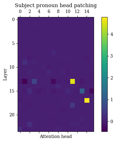
The four attention heads with the highest attributions for $n_{\text{subj}}$ are 17.14, 13.11, 15.13, and 13.3, with corrupted-clean logit differences of 4.7859, 4.5473, 1.0804, 0.6352 respectively. The four attention heads with the highest attributions for $n_{\text{obj}}$ are 17.14, 15.13, 13.11, and 22.2, with corrupted-clean logit differences of 3.5636, 3.0652, 2.1328, 0.5218 respectively. The most striking result is that the three attention heads with the largest attributions are a subset of those four heads with the highest feature norms. Of course, also striking is the absence of attention head 18.11 from the list of heads with highest attributions, despite being among the heads with highest feature norms; my suspicion is that this is due to QK circuit effects (i.e. attention head 18.11 yields outputs that would’ve contributed greatly to the observables—but it doesn’t attend to the tokens that would be responsible for those outputs).

Despite the “false positive” of attention head 18.11, seeing that feature vector norms were able to correctly predict three of the four heads with highest attribution on real data—predicting this without using any data^[6] and only using the OV circuit—was very exciting for me. My intuition regarding the use of feature vector norms, therefore, is that they can yield an inexpensive initial “ansatz” of which model components you should further investigate with more data- and computationally-intensive methods.

Cosine similarities and coupling coefficients

The next thing to look into: cosine similarities and coupling coefficients between the $n_{\text{subj}}$ feature vectors and the $n_{\text{obj}}$ feature vectors. The four heads with the highest cosine similarities between are 17.14, 18.11, 15.13, and 13.11, with cosine similarities of 0.9882, 0.9831, 0.9816, and 0.9352 respectively. Note that these cosine similarities are very close to 1 -- indicating that the model is using (approximately) the same feature vectors for predicting subject pronouns as it uses for predicting object pronouns. When I first saw these results, I was very excited: we now have evidence of a case where the model is using the same features for two different tasks! Even though subject pronoun prediction and object pronoun prediction are indeed similar, there is no guarantee that the model would use the same features for both: hence my welcome surprise at seeing otherwise.

Indeed, when we look at the cosine similarities between the pre-unembedding observables $W_U^T{n}_{\text{subj}}$ and $W_U^T{n}_{\text{obj}}$, we find that they only have a cosine similarity of 0.5685. Thus, even though the tasks are similar, they are not so inherently similar as for it to be trivial that the model would use the same features for both.

I then looked at the coupling coefficients between heads 17.14, 15.13, and 13.11 (the heads that appear in common among those with the highest cosine similarities, highest feature norms, and highest head attributions). After finding them, the next step was to record the actual dot products of all embeddings in the dataset with the $n_{\text{subj}}$ feature vectors and $n_{\text{obj}}$ feature vectors. Once this was done, then for each feature vector, I considered the ratio of $n_{\text{subj}}$ to $n_{\text{obj}}$ dot products, and found the best-fit line to fit this data. The results are given in the below table.

Head	Coupling coefficient	Cosine similarity	Best-fit line slope	$r^2$
17.14	0.67086	0.9882	0.67774	0.99811
15.13	0.77306	0.9816	0.79353	0.98146
13.11	0.73552	0.9352	0.75580	0.9274281

Notice that the coupling coefficients almost exactly match the slopes of the best-fit lines—indicating that they did indeed accurately predict the ratio of dot products.

In addition to looking at the ratio of dot products between the two vectors, we also investigated whether the coupling coefficients predicted the ratio of activation patching attribution scores between heads. The resulting scatter plot is given below: each point represents an attention head, its x-coordinate represents its coupling coefficient, and its y-coordinate represents the ratio between the mean attribution score for that head for $n_{\text{obj}}$ and the mean attention score for that head for $n_{\text{subj}}$. (Note that I excluded attention heads with attribution scores less than 0.1.)

Due to QK-circuit effects, there isn’t a perfect correlation here, as opposed to when coupling coefficients are used for predicting dot products. Nevertheless, we can see that coupling coefficients still provide a decent estimation of not only the extent to which feature vectors’ dot products will be coupled, but even the extent to which attention heads’ attributions will be coupled.

SVD

One thing that I was interested in determining: to what extent are the feature vectors obtained by observable propagation aligned with the singular vectors of weight matrices? I investigated this for the $W_{OV}$ matrices of the three attention heads considered above: 17.14, 15.13, and 13.11. The below table provides, for each head, the indices of the singular vectors that have the highest cosine similarities with the $n_{\text{subj}}$ and $n_{\text{obj}}$ feature vectors for that head, along with the cosine similarities.

Head	$n_{\text{subj}}$ vs $n_{\text{obj}}$	Top 5 singular vector indices	Top 5 absolute cosine similarities
17.14	$n_{\text{subj}}$	1, 3, 0, 2, 4	0.8169, 0.4725, 0.2932, 0.0981, 0.0827
17.14	$n_{\text{obj}}$	1, 3, 0, 4, 15	0.8052, 0.4980, 0.2758, 0.1019, 0.0394
15.13	$n_{\text{subj}}$	0, 1, 17, 28, 13	0.9466, 0.1254, 0.0875, 0.0774, 0.0747
15.13	$n_{\text{obj}}$	0, 1, 9, 65, 13	0.9451, 0.1761, 0.0761, 0.0622, 0.0597
13.11	$n_{\text{subj}}$	4, 3, 2, 1, 7	0.6470, 0.5843, 0.3451, 0.2164, 0.1508
13.11	$n_{\text{obj}}$	3, 4, 2, 7, 8	0.5982, 0.5345, 0.4869, 0.1499, 0.1007

For head 15.13, singular vector 0 was very well-aligned with the feature vectors that observable propagation finds. However, this is less the case for head 17.14 (where the top absolute cosine similarities for $n_{\text{subj}}$ and $n_{\text{obj}}$ are 0.8169 and 0.8052 respectively), and even less so for head 13.11 (where the top absolute cosine similarities for $n_{\text{subj}}$ and $n_{\text{obj}}$ are 0.6470 and 0.5982 respectively). Additionally, for heads 17.14 and 13.11 in particular, the absolute cosine similarities for singular vectors other than the most similar one are still non-negligible, indicating that one singular vector alone cannot capture the full behavior of the feature vector.

It is also worth noting that for head 13.11, the most similar singular vector for $n_{\text{subj}}$ is different from the most similar singular vector for $n_{\text{obj}}$. Since similar vectors are orthogonal, this means that naively analyzing head 13.11 by looking at the most similar singular vector for $n_{\text{subj}}$ and $n_{\text{obj}}$ would mistakenly indicate that these two observables correspond to different features (despite their feature vector cosine similarity of 0.9352).

I think that these examples demonstrate the utility of using SVD to interpret weight matrices as explored by Beren Millridge and Sid Black—but also the necessity of constructing explicit feature vectors using observable propagation, rather than only looking at the most similar singular vectors. SVD can prove useful as an initial step for interpretability, but it doesn’t tell the whole story; observable propagation’s explicit feature vectors allow for further quantitative analysis to be performed.

Activation steering

As mentioned earlier, observable propagation does not take into account the nonlinearities involved in the QK circuit of Transformers. Thus, there was a fear that the feature vectors yielded by observable propagation would be unable to accurately predict the behavior of the model in practice.

In order to test this fear, I performed some preliminary activation steering experiments: seeing if adding the feature vectors found by observable propagation to the embeddings of certain tokens could be used to change the model’s output. The idea is that if these vectors represent features that are robust even in the presence of the QK circuit, then adding these vectors should cause the model’s output to change accordingly (e.g. adding a feature vector for $n_{\text{subj}}$ to embeddings should lead to a higher output for $n_{\text{subj}}$).

I tested activation steering on the three attention heads of interest (17.14, 15.13, 13.11) for both the $n_{\text{subj}}$ and $n_{\text{obj}}$ observables. First, I used logit attribution to determine which token was most important for each head. Then, I added/​subtracted 50 times the feature vector for that attention head to the embeddings of that token^[7]. I looked at the mean difference in model output over our dataset of prompts; the results can be found in the below table.

Head	$n_{\text{subj}}$ vs $n_{\text{obj}}$	Token	$-50v$ mean difference	$+50v$ mean difference
17.14	$n_{\text{subj}}$	15	-100.780	87.517
17.14	$n_{\text{obj}}$	15	-87.038	70.865
15.13	$n_{\text{subj}}$	6	-13.238	26.132
15.13	$n_{\text{obj}}$	6	-22.681	23.150
13.11	$n_{\text{subj}}$	6	-4.111	12.659
13.11	$n_{\text{obj}}$	6	-16.343	5.992

As we can see, the feature vectors were quite effective—although more so in some attention heads than others. In addition to different strengths of effects, we also see asymmetries, in which subtracting a feature vector yields a greater effect than adding that feature vector, or vice versa. I chalk these phenomena up to QK circuit nonlinearities, along with attention head composition effects (e.g. the feature vector for head 13.11 might actually be in the opposite direction as the feature vector for virtual attention head 13.3 → 17.14 -- where the same steering vector not only affects different heads in the same layer, but even different heads later on in the computation). Nevertheless, the fact that activation steering was efficacious in this setting gives me hope for observable propagation.

Preliminary gender bias results

In addition to the work on gendered pronoun prediction, I also wanted to investigate a more “practical” problem: addressing occupational gender bias in language models. Consider the prompt template "<|endoftext|>My friend [NAME] is an excellent", where [NAME] is replaced by the names a gendered name. Now, if the name in the prompt is female, then we would expect the model to predict that the next token is more likely to be ” actress” than ” actor”—the two tokens refer to the same occupation, but the former is grammatically female, while the latter is conventionally grammatically male. This is sensible behavior from the language model.

However, the model also predicts that for a female name, the next token is more likely to be ” nurse” than ” programmer”. In this case, we say that the model is biased, because it is making a prediction on the basis of gender, even though the difference between the occupations of nursing and programming should not be related to grammatical gender.

As such, this motivates the following questions:

• Do the same features that cause the model to predict ” actress” to be more likely than ” actor” also cause the model to predict ” nurse” to be more likely than ” programmer”?

• Can we find activation steering vectors that lessen the extent to which ” nurse” is predicted over ” programmer”, while increasing the extent to which ” actress” is predicted over ” actor”?

We can begin to tackle these tasks by defining the observables of interest.$n_{\text{same}}$ will be the observable $e_{\text{" actress"}}-e_{\text{" actor"}}$, representing the extent to which the model predicts the token ” actress” over ” actor”. $n_{\text{diff}}$ will be the observable $e_{\text{" nurse"}}-e_{\text{" programmer"}}$, representing the extent to which the model predicts the token ” nurse” over ” programmer”. Ideally, the model’s outputs would be high for $n_{\text{same}}$ given female names, because this represents the model recognizing that the word “actress” is specifically applied to women; on the other hand, the model’s outputs should be low for $n_{\text{diff}}$ given female names, because otherwise, this is evidence of model bias.

Although I’m still in the process of investigating this task, here are a few preliminary results demonstrating the application of observable propagation to this setting.

The model uses some of the same features to predict $n_{\text{same}}$ as $n_{\text{diff}}$

Initially looking at the cosine similarities for attention heads’ feature vectors between $n_{\text{same}}$ and $n_{\text{diff}}$ didn’t indicate that the model was using similar features for both observables: the highest cosine similarity found was only 0.4896, for head 15.13. (Interestingly, we also found a number of heads with cosine similarities less than −0.75.)

However, I then took into account attention head composition, which bore more fruit. As one example, I found that the feature vector for $n_{\text{same}}$ corresponding to virtual attention head $6.6\to 15.13\to 17.14$ had a cosine similarity of $0.9541$ with the feature vector for $n_{\text{diff}}$ corresponding to virtual head $6.6\to 15.13\to 21.13$. Note that the cosine similarity for head 6.6, without considering any attention head composition, is $-0.0640$.

My preliminary takeaway is that when attention head composition is taken into account, the model does use some of the same features in computing its output for $n_{\text{same}}$ as it does for $n_{\text{diff}}$. In other words, some of the same information that is used to correctly predict that a female name is more likely to precede the token ” actress” than ” actor” is also used to yield the biased output that female names are more likely to be associated with the token ” nurse” than ” programmer”.

In an update, I plan to provide a more thorough analysis of shared feature vectors between the two observables. For now, though, results such as this seem to suggest that to some extent, the same intermediate computations are being used in both the desired scenario and the biased scenario.

Finding steering vectors to debias the model

I then wanted to see if I could find some steering vectors such that, when these vectors were added to certain activations, they would improve the model’s performance on the $n_{\text{same}}$ objective but decrease its performance on the $n_{\text{diff}}$ objective; this corresponds to decreasing biased behavior while increasing desired behavior.

As our steering vectors, I tried using the feature vectors from a number of different attention heads whose coupling coefficients between $n_{\text{same}}$ and $n_{\text{diff}}$ feature vectors were the most negative. Although not every head worked, I found a number of heads where adding the feature vectors for those heads did yield the desired effects. I evaluated activation steering results using the methodology from the previous activation steering experiments, using a dataset generated by inserting gendered names into the prompt template "<|endoftext|>My friend [NAME] is an excellent". The results for these heads can be found in the below table:

Head	Token	$n_{\text{diff}}$ or $n_{\text{same}}$	Coupling	Feature multiplier	$n_{\text{diff}}$ effect	$n_{\text{same}}$ effect
17.6	5	$n_{\text{diff}}$	-0.5230	-300	-3.6119	2.7614
18.2	0	$n_{\text{diff}}$	-0.2298	-1000	-0.4604	0.4694
19.15	0	$n_{\text{diff}}$	-0.4957	-300	-0.8513	1.8351
23.10	4	$n_{\text{same}}$	-0.5665	-120	-1.2027	0.1038

Note that some trial and error was used to find which attention heads yielded the best effects, along with which feature multipliers were the best. For the reasons mentioned in the discussion of the previous activation steering experiments, not every attention head worked as much as one might initially think. However, by using the heads with the most negative coupling coefficients as a guide, I was able to relatively-easily find some good steering vectors.

In particular, when I subtracted $-300$ times the feature vector for $n_{\text{diff}}$ for attention head 17.6 from the embeddings of token 5, this impressively led to a mean effect of $-3.6119$ logits for $n_{\text{diff}}$ and $2.7614$ logits for $n_{\text{same}}$. This means that after this vector was applied to the embeddings, the average prediction of the biased output was $-3.6119$ logits less than before, while the average prediction of the grammatically-correct output was 2.7614 logits more than before.

I found these preliminary activation steering results to be a nice example of the benefits that observable propagation brings. By enabling specific tasks to be mathematically formalized as observables, whose corresponding feature vectors can then be compared using metrics like coupling coefficients, the search for steering vectors that improve the model’s performance on one task while decreasing it on another can be made far simpler.

Discussion

So, given these experiments, how useful can we say that observable propagation is? The preliminary results that I’ve found so far (including those presented in this post) suggest that it’s pretty useful in at least the following ways:

• It allows for the behavior of model components to be predicted without running the model on any data, using feature vector norms and coupling coefficients. Even when there are differences between the predictions and the actual results, the predictions can nevertheless be used as a good jumping-off point for further analysis.

• It can provide a “trace” of what information is being used throughout the model for a given task.

• It lets us get a look at when the model is using the same features for multiple different tasks, allowing for a better understanding of common computations used by the model.

• It can be used as a starting point for finding activation steering vectors relevant to specific tasks, or even activation steering vectors that can have different (intended) effects on different tasks.

Of course, there are still a number of limitations to observable propagation as presented. The biggest such limitation is that observable propagation only addresses OV circuits in Transformers, ignoring all of the computation performed in QK circuits. This means, for instance, that the mechanisms behind induction heads cannot be adequately modeled. This also leads to some of the unexpected effects seen in the activation steering experiments (e.g. asymmetric effects, feature vectors being less efficacious than expected, etc.). Now, dealing with QK circuits is quite difficult, because unlike MLPs and LayerNorms, QK circuits are nonlinearities that involve multiple tokens. But in order for us to have a full understanding of Transformers, though, QK circuits must be tackled: there cannot be any ignorabimus.

Beyond this, there is also the question of the extent to which the linear approximation approach for extending observable propagation to work with MLPs can yield a tractable set of features corresponding to different nearly-linear subregions in the MLP (a la the polytope lens), or whether the nonlinearities in MLPs are so great as to make such an effort infeasible. Some preliminary experiments that didn’t make it into this post indicated MLP feature vectors for $n_{\text{subj}}$ and $n_{\text{obj}}$ with a cosine similarity of around 0.60 -- which isn’t too high. But cosine similarity might not be the right metric for measuring similarity between “local features” found via linear approximation; alternatively, a better method for finding the point at which the linear approximation is performed might have yielded more similar feature vectors. Regardless, I plan to run more experiments on larger datasets with a focus on MLP features.

Despite these limitations, I think that observable propagation represents an important first step towards deeply understanding the feature vectors that Transformers utilize in their computations, and how these feature vectors can be used to change these models’ behavior. For me at least, the results of these preliminary experiments suggest that observable propagation will prove to be a useful tool for both interpreting and steering Transformers.

As a final note, let’s return to the earlier question of what generalizations could increase the power of observable propagation that I’m failing to make. It’s hard for me to enumerate a list of my own blind spots, of course. I will say, though, that one limitation is that the “observable/​feature vector” paradigm only looks at the interaction between a single token and a feature vector, rather than the interaction between multiple tokens. But interactions between multiple tokens are necessary for understanding QK circuits, for instance. Now, in the setting of linear algebra, a natural sort of function on multiple vectors is a “multilinear form”, which generalizes the notion of a linear functional to multiple arguments. As such, one way to generalize the observable propagation paradigm, which currently only makes use of linear functionals, would be to consider multilinear forms. But the proper way to do so remains to be seen.

Conclusion

In this post, I introduce “observable propagation”, a simple method for automatically finding feature vectors in Transformers’ OV circuits that correspond to certain tasks. This post also develops a mathematical framework for analyzing these feature vectors, that allows for the prediction of model behavior on different tasks without running the model on any data. Preliminary experiments suggest that these methods perform well in predicting model behavior and steering model behavior towards desired outcomes. Of course, there’s still a lot more work to be done in testing these methods and improving them, but I think that what I’ve presented thus far in this post implies that observable propagation can already be useful.

If this post has piqued your interest, then stay tuned for an update which will contain even more experiments. Thank you for reading!

1. ^

   For those who have read ahead: this refers to finding approximate feature vectors by ignoring LayerNorms, and finding better approximations using small amounts of data by finding the linear approximation of LayerNorm at those datapoints.

2. ^

   This name is intended to suggest the notion of “observables” from quantum mechanics; in that domain, observables are Hermitian operators corresponding to certain properties of a quantum system that one wants to measure. Although there are some differences between that setting and the LLM setting (for instance, a linear functional is not a Hermitian operator), the similarities between the two cases provide valuable intuition: in both cases, an observable is a linear map that corresponds to a type of measurement of a probabalistic system.

3. ^

   Note that while linear functionals and vectors are different beasts in general, it’s true that in finite-dimensional vector spaces, there is a one-to-one natural correspondence between linear functionals and vectors. As such, for a vector $n$, I might abuse notation a bit and refer to both $n$ and $n^T$ as observables.

4. ^

   In essence, what this process is actually doing is computing the gradient of a specific computational path through the model that passes through the nonlinearity.

5. ^

   This follows from the expression for the gradient of LayerNorms used in the proof of Theorem 1.

6. ^

   Technically, the mean norms of embeddings were used in order to approximate the gradient of the final LayerNorm in the model, ln_f. But because the computational paths associated with these single attention heads all go through the same LayerNorm, we can get a decent approximation of relative feature vector norms by simply ignoring the LayerNorms entirely. I haven’t included the figures for that here, but looking at feature vector norms without taking into account LayerNorms yields the same top four attention heads.

7. ^

   There was nothing principled about multiplying the feature vector by 50, as opposed to some other constant.