interpreting GPT: the logit lens
This post relates an observation I’ve made in my work with GPT-2, which I have not seen made elsewhere.
IMO, this observation sheds a good deal of light on how the GPT-2/3/etc models (hereafter just “GPT”) work internally.
There is an accompanying Colab notebook which will let you interactively explore the phenomenon I describe here.
[Edit: updated with another section on comparing to the inputs, rather than the outputs. This arguably resolves some of my confusion at the end. Thanks to algon33 and Gurkenglas for relevant suggestions here.]
[Edit 5/17/21: I’ve recently written a new Colab notebook which extends this post in various ways:
trying the “lens” on various models from 125M to 2.7B parameters, including GPT-Neo and CTRL
exploring the contributions of the attention and MLP sub-blocks within transformer blocks/layers
trying out a variant of the “decoder” used in this post, which dramatically helps with interpreting some models
]
overview
GPT’s probabilistic predictions are a linear function of the activations in its final layer. If one applies the same function to the activations of intermediate GPT layers, the resulting distributions make intuitive sense.
This “logit lens” provides a simple (if partial) interpretability lens for GPT’s internals.
Other work on interpreting transformer internals has focused mostly on what the attention is looking at. The logit lens focuses on what GPT “believes” after each step of processing, rather than how it updates that belief inside the step.
These distributions gradually converge to the final distribution over the layers of the network, often getting close to that distribution long before the end.
At some point in the middle, GPT will have formed a “pretty good guess” as to the next token, and the later layers seem to be refining these guesses in light of one another.
The general trend, as one moves from earlier to later layers, is
“nonsense / not interpretable” (sometimes, in very early layers) -->
“shallow guesses (words that are the right part of speech / register / etc)” -->
“better guesses”
...though some of those phases are sometimes absent.
On the other hand, only the inputs look like the input tokens.
In the logit lens, the early layers sometimes look like nonsense, and sometimes look like very simple guesses about the output. They almost never look like the input.
Apparently, the model does not “keep the inputs around” for a while and gradually process them into some intermediate representation, then into a prediction.
Instead, the inputs are immediately converted to a very different representation, which is smoothly refined into the final prediction.
This is reminiscent of the perspective in Universal Transformers which sees transformers as iteratively refining a guess.
However, Universal Transformers have both an encoder and decoder, while GPT is only a decoder. This means GPT faces a tradeoff between keeping around the input tokens, and producing the next tokens.
Eventually it has to spit out the next token, so the longer it spends (in depth terms) processing something that looks like token i, the less time it has to convert it into token i+1. GPT has a deadline, and the clock is ticking.
More speculatively, this suggests that GPT mostly “thinks in predictive space,” immediately converting inputs to predicted outputs, then refining guesses in light of other guesses that are themselves being refined.
I think this might suggest there is some fundamentally better way to do sampling from GPT models? I’m having trouble writing out the intuition clearly, so I’ll leave it for later posts.
Caveat: I call this a “lens” because it is one way of extracting information from GPT’s internal activations. I imagine there is other information present in the activations that cannot be understood by looking at logits over tokens. The logit lens show us some of what is going on, not all of it.
background on GPT’s structure
You can skip or skim this if you already know it.
Input and output
As input, GPT takes a sequence of tokens. Each token is a single item from a vocabulary of N_v=50257 byte pairs (mostly English words).
As output, GPT returns a probability distribution over the vocabulary. It is trained so this distribution predicts the next token.
That is, the model’s outputs are shifted forward by one position relative to the inputs. The token at position i should, after flowing through the layers of the model, turn into the token at position i+1. (More accurately, a distribution over the token at position i+1.)
Vocab and embedding spaces
The vocab has size N_v=50257, but GPT works internally in a smaller “embedding” vector space, of dimension N_e.
For example, in the GPT-2 1558M model size, N_e=1600. (Below, I’ll often assume we’re talking about GPT-2 1558M for concreteness.)
There is an N_v-by-N_e embedding matrix W which is used to project the vocab space into the embedding space and vice versa.
In, blocks, out
The first thing that happens to the inputs is a multiplication by W, which projects them into the embedding space. [1]
The resulting 1600-dimensional vector then passes through many neural network blocks, each of which returns another 1600-dimensional vector.
At the end, the final 1600-dimensional vector is multiplied by W’s transpose to project back into vocab space.
The resulting 50257-dim vectors are treated as logits. Applying the softmax function to them gives you the output probability distribution.
the logit lens
As described above, GPT schematically looks like
Project the input tokens from vocab space into the 1600-dim embedding space
Modify this 1600-dim vector many times
Project the final 1600-dim vector back into vocab space
We have a “dictionary,” W, that lets us convert between vocab space and embedding space at any point. We know that some vectors in embedding space make sense when converted into vocab space:
The very first embedding vectors are just the input tokens (in embedding space)
The very last embedding vectors are just the output logits (in embedding space)
What about the 1600-dim vectors produced in the middle of the network, say the output of the 12th layer or the 33rd? If we convert them to vocab space, do the results make sense? The answer is yes.
logits
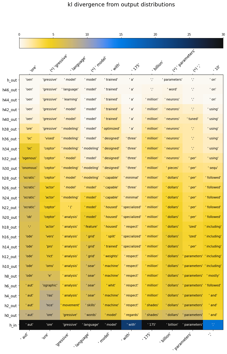
For example: the plots below show the logit lens on GPT-2 as it predicts a segment of the abstract of the GPT-3 paper. (This is a segment in the middle of the abstract; it can see all the preceding text, but I’m not visualizing the activations for it.)
For readability, I’ve made two plots showing two consecutive stretches of 10 tokens. Notes on how to read them:
The input tokens are shown as 45-degree tilted axis labels at the bottom.
The correct output (i.e. the input shifted by one) is likewise shown at the top.
A (*) is added in these labels when the model’s top guess matched the correct output.
The vertical axis indexes the layers (or “blocks”), zero-indexed from 0 to 47. To make the plots less huge I skip every other intermediate layer. The Colab notebook lets you control this skipping as you like.
The top guess for each token, according to the model’s activations at a given layer, is printed in each cell.
The colors show the logit associated with the top guess. These tend to increase steadily as the model converges on a “good guess,” then get refined in the last layers.
Cells are outlined when their top guess matches the final top guess.
For transformer experts: the “activations” here are the block outputs after layer norm, but before the learned point-wise transformation.
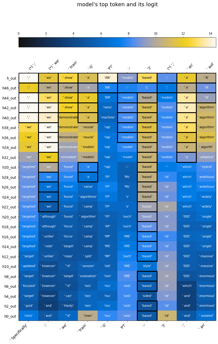
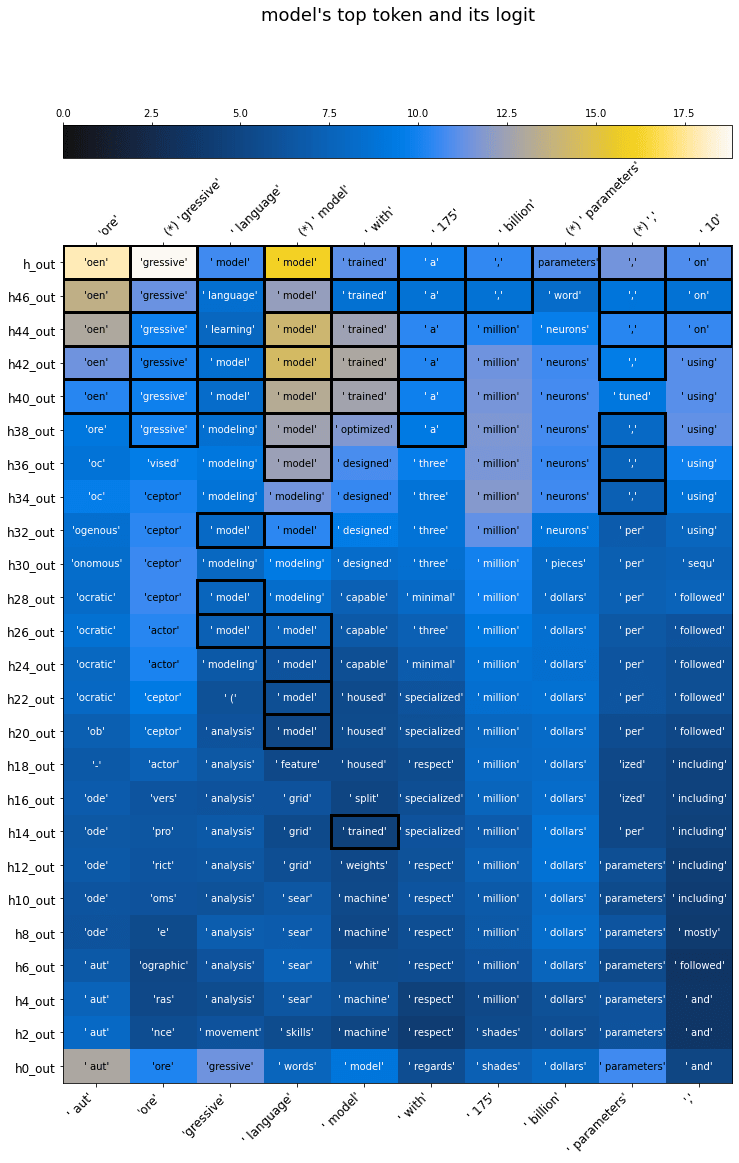
There are various amusing and interesting things one can glimpse in these plots. The “early guesses” are generally wrong but often sensible enough in some way:
“We train GPT-3...” 000? (someday!)
“GPT-3, an...” enormous? massive? (not wrong!)
“We train GPT-3, an aut...” oreceptor? (later converges to the correct oregressive)
“model with 175...” million? (later converges to a comma, not the correct billion)
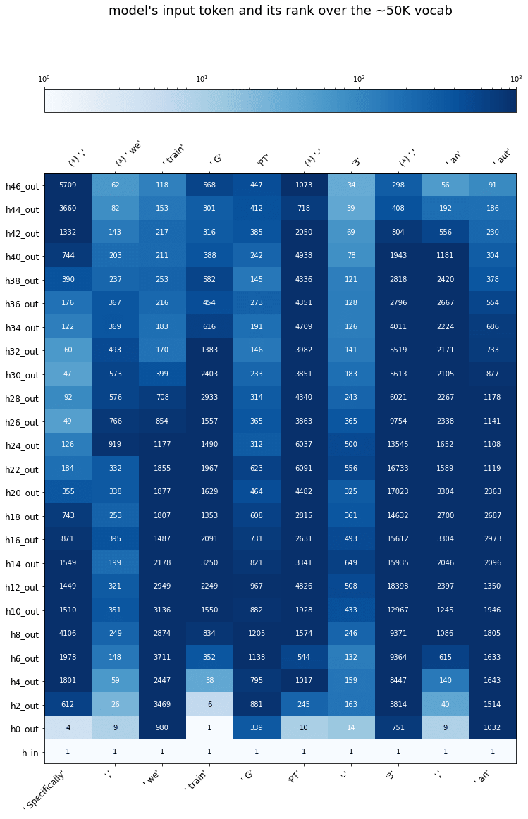
ranks
The view above focuses only on the top-1 guess at each layer, which is a reductive window on the full distributions.
Another way to look at things: we still reduces the final output to the top-1 guess, but we compare other distributions to the final one by looking at the rank of the final top-1 guess.
Even if the middle of the model hasn’t yet converged to the final answer, maybe it’s got that answer somewhere in its top 3, top 10, etc. That’s a lot better than “top 50257.”
Here’s the same activations as ranks. (Remember: these are ranks of the model’s final top-1 prediction, not the true token.)
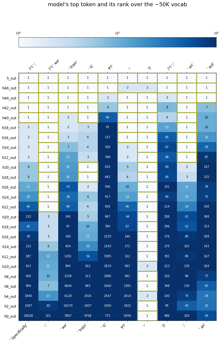
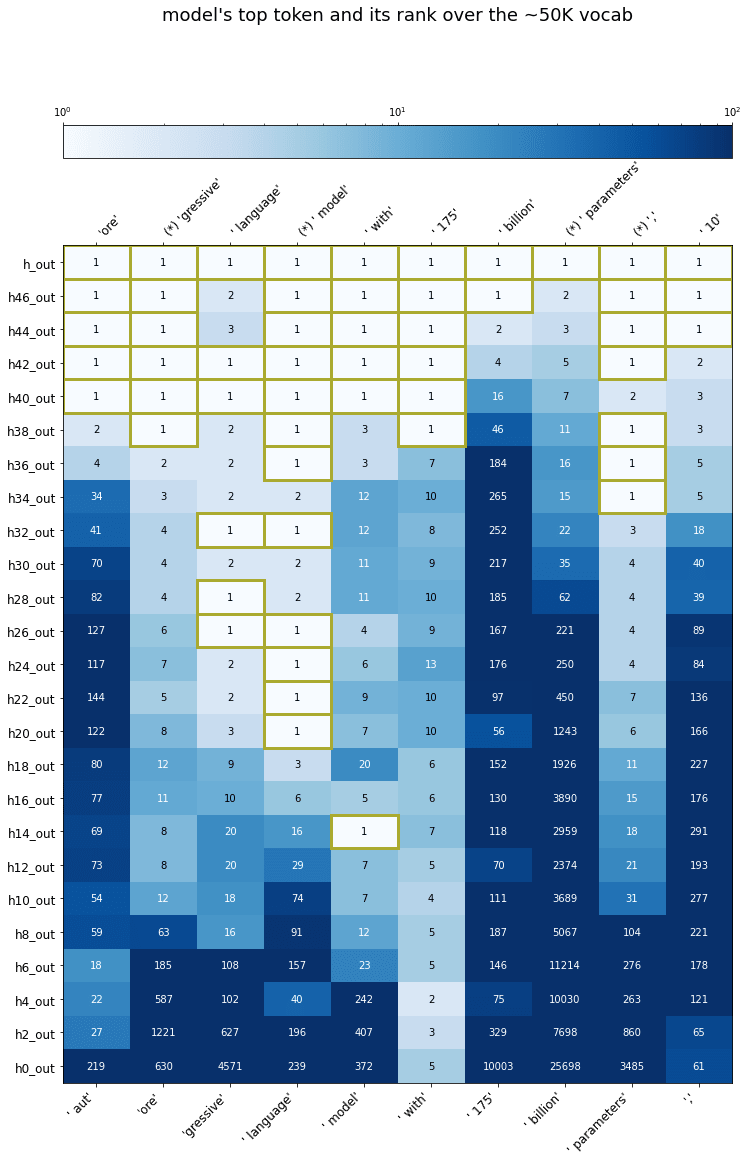
In most cases, network’s uncertainty has drastically reduced by the middle layers. The order of the top candidates may not be right, and the probabilities may not be perfectly calibrated, but it’s got the gist already.
KL divergence and input discarding
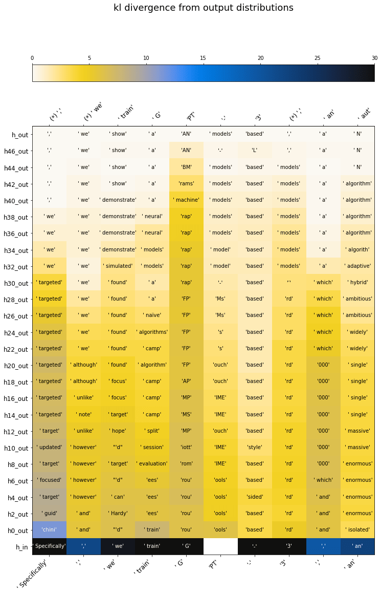
Another way of comparing the similarity of two probability distributions is the KL divergence. Taking the KL divergence of the intermediate probabilities w/r/t the final probabilities, we get a more continuous view of how the distributions smoothly converge to the model’s output.
Because KL divergence is a more holistic measure of the similarity between two distributions than the ones I’ve used above, it’s also my preferred metric for making the point that nothing looks like the input.
In the plots above, I’ve skipped the input layer (i.e. the input tokens in embedding space). Why? Because they’re so different from everything else, they distract the eye!
In the plots below, where color is KL divergence, I include the input as well. If we trust that KL divergence is a decent holistic way to compare two distributions (I’ve seen the same pattern with other metrics), then:
Immediately, after the very first layer, the input has been transformed into something that looks more like the final output (47 layers layer) than it does like the input.
After this one discontinuous jump, the distribution progresses in a much more smooth way to the final output distribution.
other examples
I show several other examples in the Colab notebook. I’ll breeze through a few of them here.
copying a rare token
Sometimes it’s clear that the next token should be a “copy” of an earlier token: whatever arbitrary thing was in that slot, spit it out again.
If this is a token with relatively low prior probability, one would think it would be useful to “keep it around” from the input so later positions can look at it and copy it. But as we saw, the input is never “kept around”!
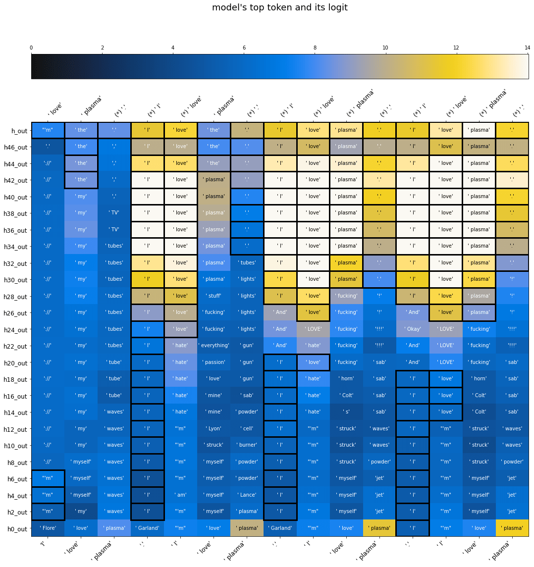
What happens instead? I tried this text:
Sometimes, when people say plasma, they mean a state of matter. Other times, when people say plasma
As shown below (truncated to the last few tokens for visibility), the model correctly predicts “plasma” at the last position, but only figures it out in the very last layers.
Apparently it is keeping around a representation of the token “plasma” with enough resolution to copy it . . . but it only retrieves this representation at the end! (In the rank view, the rank of plasma is quite low until the very end.)
This is surprising to me. The repetition is directly visible in the input: “when people say” is copied verbatim. If you just applied the rule “if input seems to be repeating, keep repeating it,” you’d be good. Instead, the model scrambles away the pattern, then recovers it later through some other computational route.
extreme repetition
We’ve all seen GPT sampling get into a loop where text repeats itself exactly, over and over. When text is repeating like this, where is the pattern “noticed”?
At least in the following example, it’s noticed in the upper half of the network, while the lower half can’t see it even after several rounds of repetition.
why? / is this surprising?
First, some words about why this trick can even work at all.
One can imagine models that perform the exact same computation as GPT-2, for which this trick would not work. For instance, each layer could perform some arbitrary vector rotation of the previous one before doing anything else to it. This would preserve all the information, but the change of basis would prevent the vectors from making sense when multiplied by W^T.
Why doesn’t the model do this? Two relevant facts:
1. Transformers are residual networks. Every connection in them looks like x + f(x) where f is the learned part. So the identity is very easy to learn.
This tends to keep things in the same basis across different layers, unless there’s some reason to switch.
2. Transformers are usually trained with weight decay, which is almost the same thing as L2 regularization. This encourages learned weights to have small L2 norm.
That means the model will try to “spread out” a computation across as many layers as possible (since the sum-of-squares is less than the square-of-sums). Given the task of turning an input into an output, the model will generally prefer changing the input a little, then a little more, then a little more, bit by bit.
1+2 are a good story if you want to explain why the same vector basis is used across the network, and why things change smoothly. This story would render the whole thing unsurprising . . . except that the input is discarded in such a discontinuous way!
I would have expected a U-shaped pattern, where the early layers mostly look like the input, the late layers mostly look like the output, and there’s a gradual “flip” in the middle between the two perspectives. Instead, the input space immediately vanishes, and we’re in output space the whole way.
Maybe there is some math fact I’m missing here.
Or, maybe there’s some sort of “hidden” invertible relationship between
the embedding of a given token, and
the model’s prior for what token comes after it (given no other information)
so that a token like “plasma” is kept around from the input—but not in the form “the output is plasma,” instead in the form “the output is [the kind of word that comes after plasma].”
However, I’m not convinced by that story as stated. For one thing, GPT layers don’t share their weights, so the mapping between these two spaces would have to be separately memorized by each layer, which seems costly. Additionally, if this were true, we’d expect the very early activations to look like naive context-less guesses for the next token. Often they are, but just as often they’re weird nonsense like “Garland.”
addendum: more on “input discarding”
In comments, Gurkenglas noted that the plots showing KL(final || layer) don’t tend the whole story.
The KL divergence is not a metric: it is not symmetric and does not obey the triangle inequality. Hence my intuitive picture of the distribution “jumping” from the input to the first layer, then smoothly converging to the final layer, is misleading: it implies we are measuring distances along a path through some space, but KL divergence does not measure distance in any space.
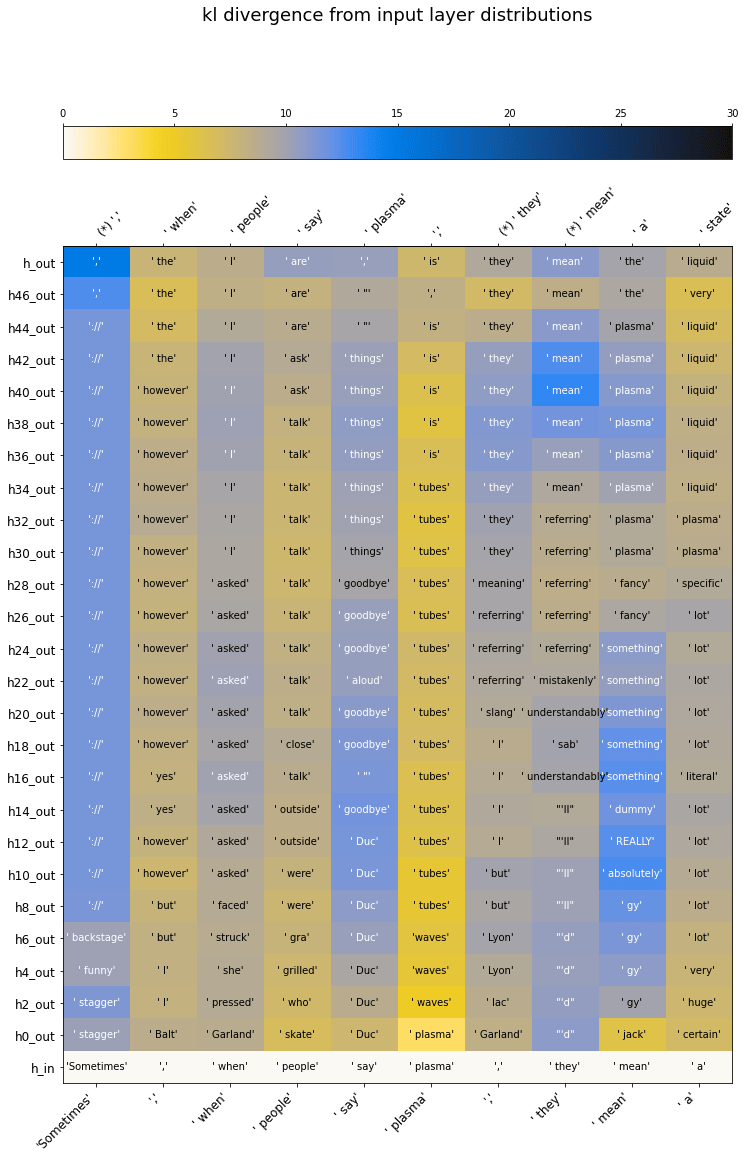
Gurkenglas and algon33 suggested plotting the KL divergences of everything w/r/t the input rather than the output: KL(input || layer).
Note that the input is close to a distribution that just assigns probability 1 to the input token (“close” because W * W^T is not invertible), so this is similar to asking “how probable is the input token, according to each layer?” That’s a question which is also natural to answer by plotting ranks: what rank is assigned to the input token by each layer?
Below, I show both: KL(input || layer), and the rank of the input token according to later layers.
For KL(input || layer), I use the same color scale as in the plots for KL(final || layer), so the two are comparable.
For the ranks, I do not use the same color scale: I have the colors bottom out at rank 1000 instead of rank 100. This gives more visual insight into where the model could be preserving input information.
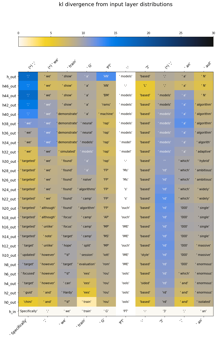
There is still a fast jump in KL(input || layer) after the input.
However, it’s far smaller than the jump in KL(output || layer) at the same point.
Note that the darkest color, meaning KL=30 does not appear on the plot of KL(input || layer).
On the plot of KL(output || layer), however, the maximum values were in fact much greater than 30; I cut off the color scale at 30 so other distinctions were perceptible at all.
Likewise, while ranks jump quickly after the input, they often stay relatively high in the context of a ~50K vocab.
I am curious about the differences here: some tokens are “preserved” much more in this sense than others.
This is apparently contextual, not just based on the token itself. Note the stark differences between the rank trajectories of the first, second, and third commas in the passage.
It’s possible that the relatively high ranks—in the 100s or 1000s, but not the 10000s—of input tokens in many cases is (related to) the mechanism by which the model “keeps around” rarer tokens in order to copy them later.
As some evidence for this, I will show plots like the above for the plasma example. Here, I show a segment including the first instance of “plasma,” rather than the second which copies it.
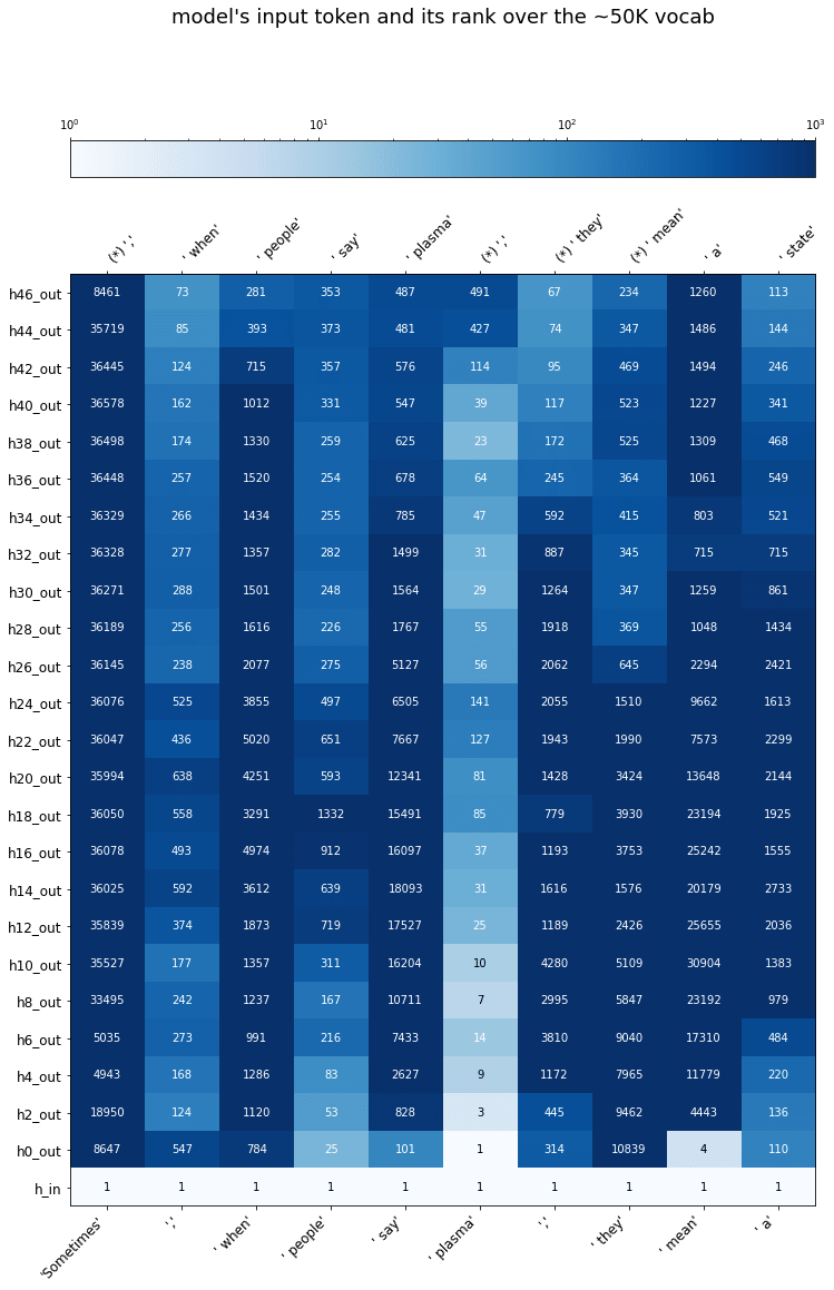
The preservation of “plasma” here is striking.
My intuitive guess is that the rarity, or (in some sense) “surprisingness,” of the token causes early layers to preserve it: this would provide a mechanism for providing raw access to rare tokens in the later layers, which otherwise only be looking at more plausible tokens that GPT had guessed for the corresponding positions.
On the other hand, this story has trouble explaining why “G” and “PT” are not better preserved in the GPT3 abstract plots just above. This is the first instance of “GPT” in the full passage, so the model can’t rely on copies of these at earlier positions. That said, my sense of scale for “well-preservedness” is a wild guess, and these particular metrics may not be ideal for capturing it anyway.
Right after this, positional embeddings are added. I’m ignoring positional embeddings in the post, but mention them in this footnote for accuracy. ↩︎
- Against Almost Every Theory of Impact of Interpretability by (17 Aug 2023 18:44 UTC; 336 points)
- The Singular Value Decompositions of Transformer Weight Matrices are Highly Interpretable by (28 Nov 2022 12:54 UTC; 200 points)
- Inside the mind of a superhuman Go model: How does Leela Zero read ladders? by (1 Mar 2023 1:47 UTC; 159 points)
- Activation Oracles: Training and Evaluating LLMs as General-Purpose Activation Explainers by (18 Dec 2025 20:21 UTC; 154 points)
- An Extremely Opinionated Annotated List of My Favourite Mechanistic Interpretability Papers v2 by (7 Jul 2024 17:39 UTC; 146 points)
- We Found An Neuron in GPT-2 by (11 Feb 2023 18:27 UTC; 143 points)
- Small Models Can Introspect, Too by (21 Dec 2025 22:20 UTC; 124 points)
- Deep learning models might be secretly (almost) linear by (24 Apr 2023 18:43 UTC; 117 points)
- Open Source Sparse Autoencoders for all Residual Stream Layers of GPT2-Small by (2 Feb 2024 6:54 UTC; 103 points)
- Knowledge Neurons in Pretrained Transformers by (17 May 2021 22:54 UTC; 100 points)
- Searching for Search by (28 Nov 2022 15:31 UTC; 98 points)
- Sparsify: A mechanistic interpretability research agenda by (3 Apr 2024 12:34 UTC; 97 points)
- Latent Introspection (and other open-source introspection papers) by (24 Mar 2026 21:23 UTC; 96 points)
- AuditBench: Evaluating Alignment Auditing Techniques on Models with Hidden Behaviors by (10 Mar 2026 19:31 UTC; 81 points)
- Language Models Use Trigonometry to Do Addition by (5 Feb 2025 13:50 UTC; 80 points)
- Gears-Level Mental Models of Transformer Interpretability by (29 Mar 2022 20:09 UTC; 76 points)
- 2020 Review Article by (14 Jan 2022 4:58 UTC; 74 points)
- How transparent is DiffusionGemma (and why it matters) by (20 Jun 2026 20:05 UTC; 73 points)
- (OLD) An Extremely Opinionated Annotated List of My Favourite Mechanistic Interpretability Papers by (18 Oct 2022 21:08 UTC; 72 points)
- Understanding SAE Features with the Logit Lens by (11 Mar 2024 0:16 UTC; 71 points)
- Narrow finetuning is different by (5 Aug 2025 14:29 UTC; 70 points)
- Eliciting secret knowledge from language models by (2 Oct 2025 20:57 UTC; 69 points)
- Mechanistically interpreting time in GPT-2 small by (16 Apr 2023 17:57 UTC; 68 points)
- Open Source Automated Interpretability for Sparse Autoencoder Features by (30 Jul 2024 21:11 UTC; 67 points)
- ‘Fundamental’ vs ‘applied’ mechanistic interpretability research by (23 May 2023 18:26 UTC; 65 points)
- Transparency and AGI safety by (11 Jan 2021 18:51 UTC; 54 points)
- How I’m thinking about GPT-N by (17 Jan 2022 17:11 UTC; 54 points)
- Narrow Finetuning Leaves Clearly Readable Traces in Activation Differences by (5 Sep 2025 12:11 UTC; 54 points)
- The Stochastic Parrot Hypothesis is debatable for the last generation of LLMs by (7 Nov 2023 16:12 UTC; 52 points)
- Othello-GPT: Future Work I Am Excited About by (29 Mar 2023 22:13 UTC; 48 points)
- Understanding mesa-optimization using toy models by (7 May 2023 17:00 UTC; 46 points)
- Understanding LLMs: Insights from Mechanistic Interpretability by (30 Aug 2025 16:50 UTC; 45 points)
- AXRP Episode 19 - Mechanistic Interpretability with Neel Nanda by (4 Feb 2023 3:00 UTC; 45 points)
- Can we interpret latent reasoning using current mechanistic interpretability tools? by (22 Dec 2025 16:56 UTC; 44 points)
- Decoding intermediate activations in llama-2-7b by (21 Jul 2023 5:35 UTC; 39 points)
- Architectures for Increased Externalisation of Reasoning by (26 Nov 2025 20:24 UTC; 38 points)
- Representation Tuning by (27 Jun 2024 17:44 UTC; 35 points)
- 's comment on (The) Lightcone is nothing without its people: LW + Lighthaven’s big fundraiser by (6 Dec 2024 2:39 UTC; 34 points)
- Machine Unlearning Evaluations as Interpretability Benchmarks by (23 Oct 2023 16:33 UTC; 33 points)
- Intervening in the Residual Stream by (22 Feb 2023 6:29 UTC; 30 points)
- Quick Thoughts on Scaling Monosemanticity by (23 May 2024 16:22 UTC; 28 points)
- Useful starting code for interpretability by (13 Feb 2024 23:13 UTC; 26 points)
- on “learning to summarize” by (12 Sep 2020 3:20 UTC; 25 points)
- What Environment Properties Select Agents For World-Modeling? by (23 Jul 2022 19:27 UTC; 25 points)
- 's comment on larger language models may disappoint you [or, an eternally unfinished draft] by (3 Dec 2021 20:19 UTC; 20 points)
- An Extremely Opinionated Annotated List of My Favourite Mechanistic Interpretability Papers by (EA Forum; 18 Oct 2022 21:23 UTC; 19 points)
- Identifying semantic neurons, mechanistic circuits & interpretability web apps by (13 Apr 2023 11:59 UTC; 18 points)
- Training a Transformer to Compose One Step Per Layer (and Proving It) by (26 Apr 2026 23:45 UTC; 17 points)
- An information-theoretic study of lying in LLMs by (2 Aug 2024 10:06 UTC; 17 points)
- My SERI MATS Application by (30 May 2022 2:04 UTC; 16 points)
- 's comment on Knowledge Neurons in Pretrained Transformers by (19 May 2021 10:42 UTC; 15 points)
- Cataloguing Priors in Theory and Practice by (13 Oct 2022 12:36 UTC; 13 points)
- 200 COP in MI: Techniques, Tooling and Automation by (6 Jan 2023 15:08 UTC; 13 points)
- 's comment on silentbob’s Shortform by (18 May 2025 20:01 UTC; 11 points)
- A “Scaling Monosemanticity” Explainer by (29 Jun 2024 17:50 UTC; 10 points)
- Task vectors & analogy making in LLMs by (8 Jan 2024 15:17 UTC; 9 points)
- 's comment on Simulacra are Things by (9 Jan 2023 3:45 UTC; 6 points)
- Exploring the Evolution and Migration of Different Layer Embedding in LLMs by (8 Mar 2024 15:01 UTC; 6 points)
- Subspace Rerouting: Using Mechanistic Interpretability to Craft Adversarial Attacks against Large Language Models by (18 Mar 2025 17:55 UTC; 6 points)
- Exploring belief states in LLM chains of thought by (27 Sep 2025 1:09 UTC; 6 points)
- Visualizing neural network planning by (9 May 2024 6:40 UTC; 4 points)
- Progress Report 4: logit lens redux by (8 Apr 2022 18:35 UTC; 4 points)
- 's comment on Evaluating the historical value misspecification argument by (30 Oct 2023 18:34 UTC; 4 points)
- Exploring vocabulary alignment of neurons in Llama-3.2-1B by (7 Jun 2025 11:20 UTC; 4 points)
- 's comment on anaguma’s Shortform by (15 Jan 2026 22:25 UTC; 4 points)
- 's comment on A Walkthrough of Interpretability in the Wild (w/ authors Kevin Wang, Arthur Conmy & Alexandre Variengien) by (8 Nov 2022 14:54 UTC; 3 points)
- 's comment on axelcore’s Shortform by (20 May 2026 17:26 UTC; 3 points)
- 's comment on DL towards the unaligned Recursive Self-Optimization attractor by (19 Dec 2021 1:36 UTC; 3 points)
- Intrinsic Dimension of Prompts in LLMs by (14 Feb 2025 19:02 UTC; 3 points)
- 's comment on No convincing evidence for gradient descent in activation space by (13 Apr 2023 4:49 UTC; 2 points)
- Mechanistic interpretability of LLM analogy-making by (20 Oct 2023 12:53 UTC; 2 points)
- 's comment on Classifying representations of sparse autoencoders (SAEs) by (17 Nov 2023 14:31 UTC; 1 point)
Unroll the sampling process: hook up all the individual GPT instances into a single long model, bypass the discretizing/embedding layers to make it differentiable end-to-end, and do gradient ascent to find the sequence which maximizes likelihood conditional on the fixed input.
Interesting, but not (I think?) the direction I was headed in.
I was thinking more about the way the model seems to be managing a tradeoff between preserving the representation of token i and producing the representation of token i+1.
The depth-wise continuity imposed by weight decay means late layers are representing something close to the final output—in late layers the model is roughly looking at its own guesses, even if they were wrong, which seems suboptimal.
Consider this scenario:
The model does poorly at position i, assigning very low probability to the true token residing at i+1.
To retain a clear view of the input sequence, the model now needs to “keep around” the true token at i+1, since its own guess is a poor proxy.
But early layers don’t know that: they can’t “look up” and notice the poor prediction. So they just treat i+1 like any other position. (I.e. there’s no way to implement a selective “copy when we got it wrong” mechanism)
In late layers, position i+1 has been converted into a guess about i+2 by the earlier layers, so we can’t rely on it to tell us what really occupied i+1.
And position i has been converted to a bad guess about position i+1, so if we use it as a proxy for i+1 we’ll do poorly.
My sampling idea was something like “let’s replace (or interpolate) late activations with embeddings of the actual next token, so the model can see what really happened, even when its probability was low.” (This is for sampling specifically because it’d be too slow in training, where you want to process a whole window at once with matrix operations; sampling has to be a loop anyway, so there’s no cost to adding stuff that only works as a loop.)
But, thinking about it more, the model clearly can perform well in scenarios like the above, e.g. my plasma example and also many other cases naturally arising in language which GPT handles well.
I have no idea how it does it—indeed the connection structure feels weirdly adverse to such operations—but apparently it does. So it’s probably premature to assume it can’t do this well, and attempt to “help it out” with extra tricks.
How far away is this from being implementable?
It doesn’t sound hard at all. The things Gwern is describing are the same sort of thing that people do for interpretability where they, eg, find an image that maximizes the probability of the network predicting a target class.
Of course, you need access to the model, so only OpenAI could do it for GPT-3 right now.
Doing it with GPT-3 would be quite challenging just for compute requirements like RAM. You’d want to test this out on GPT-2-117M first, definitely. If the approach works at all, it should work well for the smallest models too.
This is very neat. I definitely agree that I find the discontinuity from the first transformer block surprising. One thing which occurred to me that might be interesting to do is to try and train a linear model to reconstitute the input from the activations at different layers to get an idea of how the model is encoding the input. You could either train one linear model on data randomly sampled from different layers, or a separate linear model for each layer, and then see if there are any interesting patterns like whether the accuracy increases or decreases as you get further into the model. You could also see if the resulting matrix has any relationship to the embedding matrix (e.g. are the two matrices farther apart or closer together than would be expected by chance?). One possible hypothesis that this might let you test is whether the information about the input is being stored indirectly via what the model’s guess is given that input or whether it’s just being stored in parts of the embedding space that aren’t very relevant to the output (if it’s the latter, the linear model should put a lot of weight on basis elements that have very little weight in the embedding matrix).
That’s a great idea!
Hmm… I guess there is some reason to think the basis elements have special meaning (as opposed to the elements of any other basis for the same space), since the layer norm step operates in this basis.
But I doubt there are actually individual components the embedding cares little about, as that seems wasteful (you want to compress 50K into 1600 as well as you possibly can), and if the embedding cares about them even a little bit then the model needs to slot in the appropriate predictive information, eventually.
Thinking out loud, I imagine there might be pattern where embeddings of unlikely tokens (given the context) are repurposed in the middle for computation (you know they’re near-impossible so you don’t need to track them closely), and then smoothly subtracted out at the end. There’s probably a way to check if that’s happening.
Thanks! I’d be quite excited to know what you find if you end up trying it.
I wasn’t thinking you would do this with the natural component basis—though it’s probably worth trying that also—but rather doing some sort of matrix decomposition on the embedding matrix to get a basis ordered by importance (e.g. using PCA or NMF—PCA is simpler though I know NMF is what OpenAI Clarity usually uses when they’re trying to extract interpretable basis elements from neural network activations) and then seeing what the linear model looks like in that basis. You could even just do something like what you’re saying and find some sort of basis ordered by the frequency of the tokens that each basis element corresponds to (though I’m not sure exactly what the right way would be to generate such a basis).
I also thought of PCA/SVD, but I imagine matrix decompositions like these would be misleading here.
What matters here (I think) is not some basis of N_emb orthogonal vectors in embedding space, but some much larger set of ~exp(N_emb) almost orthogonal vectors. We only have 1600 degrees of freedom to tune, but they’re continuous degrees of freedom, and this lets us express >>1600 distinct vectors in vocab space as long as we accept some small amount of reconstruction error.
I expect GPT and many other neural models are effectively working in such space of nearly orthogonal vectors, and picking/combining elements of it. A decomposition into orthogonal vectors won’t really illuminate this. I wish I knew more about this topic—are there standard techniques?
You might want to look into NMF, which, unlike PCA/SVD, doesn’t aim to create an orthogonal projection. It works well for interpretability because its components cannot cancel each other out, which makes its features more intuitive to reason about. I think it is essentially what you want, although I don’t think it will allow you to find directly the ‘larger set of almost orthogonal vectors’ you’re looking for.
Related layer visualizations: “Looking for Grammar in All The Right Places”.
I just found the paper BERT’s output layer recognizes all hidden layers? Some Intriguing Phenomena and a simple way to boost BERT, which precedes this post by a few months and invents essentially the same technique as the logit lens.
So consider also citing that paper when citing this post.
As an aside, I would guess that this is the most cited LessWrong post in the academic literature, but it would be cool if anyone had stats on that.
Maybe I am misunderstanding something, but to me it is very intuitive that there is a big jump from the embedding output to the first transformer block output. The embedding is backpropagated into so it makes sense to see all representations as representations of the prediction we are trying to make, i.e. of the next word.
But the embedding is a prediction of the next word based on only a single word, the word that is being embedded. So the prediction of the next word is by necessity very bad (the BPE ensures that, IIUC, because tokens that would always follow one another are merged).
The first transformer block integrates hundreds of words of context into the prediction, that’s where the big jump comes from.
Is it really trained to output the input offset by one, or just to have the last slot contain the next word? Because I would expect it to be better at copying the input over by one...
If each layer were trained to give its best guess at the next token, this myopia would prevent all sorts of hiding data for later. This would be a good experiment for your last story, yes? I expect this would perform very poorly, though if it doesn’t, hooray, for I really don’t expect that version to develop inner optimizers.
I think I understand your question and was also confused by this for a bit so I wanted add in some points of clarification. First I want out that I really couldn’t find a satisfactory explanation of this particular detail (at least one that I could understand) so I pieced this together myself from looking at the huggingface code for GPT2. I may get some details wrong.
During training at each step the GPT2 takes in an N tokens and outputs N tokens. But the i-th output token is computed in such away that it only relies on the information from tokens 1, …, i and is meant to predict i+1-th token from these. I think it’s best to think of each output being computed independently of the others (though this isn’t strictly true since the separate outputs are computed by shared matrices). So for each i, we train the network so that the i-th output produces the correct result given the _input_ tokens 1, …, i. There is a term in the loss function for each output token and the total loss is the sum of all the losses of the output tokens. The outputs at other positions do not play a role in the i-th output token, only the first 1,..., i input tokens do.
During inference, given an input of k tokens, we are only concerned with the k-th output token (which should predict the token following the first k). GPT-3 also produces predictions for the outputs before position k but these are just ignored since we already know what these values should be.
Not sure I understand the distinction, could you rephrase?
If by “last slot” you mean last layer (as opposed to earlier layers), that seems like the same thing as outputting the input offset by one.
If by “last slot” you mean the token N+1 given tokens (1, 2, … N), then no, that’s not how GPT works. If you put in tokens (1, 2, … N), you always get guesses for tokens (2, 3, …, N+1) in response. This is true even if all you care about is the guess for N+1.
I meant your latter interpretation.
Can you measure the KL-divergence at each layer from the input, rather than the output? KL does not satisfy the triangle inequality, so maybe most of the layers are KL-close to both input and output?
GPT uses ReLU, yes? Then the regularization would make it calculate using small values, which would be possible because ReLU is nonlinear on small values. If we used an activation function that’s linear on small values, I would therefore expect more of the calculation to be visible.
One can do this in the Colab notebook by calling
show_token_progresswithcomparisons_vs="first"rather than the default"final". IIRC, this also shows a discontinuous flip at the bottom followed by slower change.(This is similar to asking the question “do the activations assign high or low probability the input token?” One can answer the same question by plotting logits or ranks with the input layer included.)
It uses gelu, but gelu has the same property. However, note that I am extracting activations right after the application of a layer norm operation, which shifts/scales the activations to mean 0 and L2 norm 1 before passing them to the next layer.
Actually, gelu is differentiable at 0, so it is linear on close-to-zero values.
Ah, I think we miscommunicated.
I meant “gelu(x) achieves its maximum curvature somewhere near x=0.”
People often interpret relu as a piecewise linear version of functions like elu and gelu, which are curved near x=0 and linear for large |x|. In this sense gelu is like relu.
It sounds like you were, instead, talking about the property of relu that you can get nonlinear behavior for arbitrarily small inputs.
This is indeed unique to relu—I remember some DeepMind (?) paper that used floating point underflow to simulate relu, and then made NNs out of just linear floating point ops. Obviously you can’t simulate a differentiable function with that trick.
(OpenAI?)
Oh that’s not good. Looks like we’d need a version of float that keeps track of an interval of possible floats (by the two floats at the end of the interval). Then we could simulate the behavior of infinite-precision floats so long as the network keeps the bounds tight, and we could train the network to keep the simulation in working order. Then we could see whether, in a network thus linear at small numbers, every visibly large effect has a visibly large cause.
By the way—have you seen what happens when you finetune GPT to reinforce this pattern that you’re observing, that every entry of the table, not just the top right one, predicts an input token?
Maybe edit the post so you include this? I know I was wondering about this too.
Post has been now updated with a long-ish addendum about this topic.
Good idea, I’ll do that.
I know I’d run those plots before, but running them again after writing the post felt like it resolved some of the mystery. If our comparison point is the input, rather than the output, the jump in KL/rank is still there but it’s smaller.
Moreover, the rarer the input token is, the more it seems to be preserved in later layers (in the sense of low KL / low vocab rank). This may be how tokens like “plasma” are “kept around” for later use.
Consider also trying the other direction—after all, KL is asymmetric.
One more reason on why this is suprising, is that other experiments found that this behaviour (forgetting then recalling) is common in MLM (masked language models) but not in simple language models like GPT-2 (see this blog post and more specifically this graph). The intepretation is that “for MLMs, representations initially acquire information about the context around the token, partially forgetting the token identity and producing a more generalized token representation; the token identity then gets recreated at the top layer” (citing from the blog post).
However, the logit lense here seems indicating that this may happen in GPT-2 (large) too. Could this be a virtue of scale? Where the same behaviour that one obtains with a MLM is reached by a LM as well with sufficient scale?
Are these known facts? If not, I think there’s a paper in here.
In all of this, there seems to be an implicit assumption that the ordering of the embedding dimensions is consistent across layers, in the sense that “dog” is more strongly associated with dimension 12 in layers 2, 3, 4, etc.
I don’t see any reason why this should be the case from either a training or model structure perspective. How, then, does the logit lens (which should clearly not be invariant with regard to a permutation of its inputs) still produce valid results for some intermediate layers?
Because the model has residual connections.
Ah, got it. Thanks a ton!
Cool project. There were some changes in HuggingFace’s transformer package which are affecting you Colab implementation. See here:
https://github.com/huggingface/transformers/issues/29576
47 layers later ?
Could you try a prompt that tells it to end a sentence with a particular word, and see how that word casts its influence back over the sentence? I know that this works with GPT-3, but I didn’t really understand how it could.
Interesting topic! I’m not confident this lens would reveal much about it (vs. attention maps or something), but it’s worth a try.
I’d encourage you to try this yourself with the Colab notebook, since you presumably have more experience writing this kind of prompt than I do.
Hey I’m not finished reading this yet but I noticed something off about what you said.
This isn’t quite right. They don’t multiply by W’s transpose at the end. Rather there is a completely new matrix at the end, whose shape is the same as the transpose of W.
You can see this in huggingface’s code for GPT2. In the class GPT2LMHeadModel the final matrix multiplication is performed by the matrix called “lm_head”, where as the matrix you call W which is used to map 50,257 dimensional vectors into 1600 dimensional space is called “wte” (found in the GPT2Model class). You can see from the code that wte has shape “Vocab size x Embed Size” while lm_head has shape “Embed Size x Vocab size” so lm_head does have the same shape as W transpose but doesn’t have the same numbers.
Edit: I could be wrong here, though. Maybe lm_head was set to be equal to wte transpose? I’m looking through the GPT-2 paper but don’t see anything like that mentioned.
Yes, this is the case in GPT-2. Perhaps the huggingface implementation supports making these two matrices different, but they are the same in the official GPT-2.
In OpenAI’s tensorflow code, see lines 154 and 171 of src/model.py. The variable “wte” is defined on 151, then re-used on 171.
In the original GPT paper, see eqs. (2) in section 3.1. The same matrix W_e is used twice. (The GPT-2 and GPT-3 papers just refer you back to the GPT paper for architecture details, so the GPT paper is the place to look.)
Edit: I think the reason this is obscured in the huggingface implementation is that they always distinguish the internal layers of a transformer from the “head” used to convert the final layer outputs into predictions. The intent is easy swapping between different “heads” with the same “body” beneath.
This forces their code to allow for heads that differ from the input embedding matrix, even when they implement models like GPT-2 where the official specification says they are the same.
Edit2: might as well say explicitly that I find the OpenAI tensorflow code much more readable than the huggingface code. This isn’t a critique of the latter; it’s trying to support every transformer out there in a unified framework. But if you only care about GPT, this introduces a lot of distracting abstraction.
Thanks for the info.
This was a great read, very informative.