How to game the METR plot
TL;DR: In 2025, we were in the 1-4 hour range, which has only 14 samples in METR’s underlying data. The topic of each sample is public, making it easy to game METR horizon length measurements for a frontier lab, sometimes inadvertently. Finally, the “horizon length” under METR’s assumptions might be adding little information beyond benchmark accuracy. None of this is to criticize METR—in research, its hard to be perfect on the first release. But I’m tired of what is being inferred from this plot, pls stop!
14 prompts ruled AI discourse in 2025
The METR horizon length plot was an excellent idea: it proposed measuring the length of tasks models can complete (in terms of estimated human hours needed) instead of accuracy. I’m glad it shifted the community toward caring about long-horizon tasks. They are a better measure of automation impacts, and economic outcomes (for example, labor laws are often based on number of hours of work).
However, I think we are overindexing on it, far too much. Especially the AI Safety community, which based on it, makes huge updates in timelines, and research priorities. I suspect (from many anecdotes, including roon’s) the METR plot has influenced significant investment decisions, but I’ve not been in any boardrooms.
Here is the problem with this. In 2025, according to this plot, frontier AI progress occurred in the regime between a horizon length of 1 to 4 hours.
Guess how many samples have 1-4hr estimated task lengths?
Just 14. How do we know? Kudos to the authors, the paper has this information, and they transparently provide task metadata.
Hopefully, for many, this alone rings alarm bells. Under no circumstance should we be making such large inferences about AGI timelines, US vs China, Closed vs Open model progress, research priorities, individual model quality etc. based on just 14 samples. An early sign of this problem was there when the original METR paper was released in March 2025. The best performing model at the time, Claude 3.7 Sonnet, was estimated to have a horizon length of 59 mins. Now see its success rate distribution over task lengths:
Notice how the model has almost a 60 ±15% probability of success on 1-2hr tasks. So why is the estimated 50% success horizon length 59 minutes?! Because it doesn’t get anything right in the 2-4 hr range. METR calculates the horizon length by fitting a logistic curve to individual sample outcomes, like the dark purple line above. Notice how 0% on the 2-4hr range leads to a very bad logistic fit (the curve is below the 95% confidence interval for 0.5-1hr, and 1hr-2hrs range). We’ll come to my skepticism arising from the core modelling assumption, of using a logistic curve, later. My suspicion is Claude 3.7 Sonnet has 0% success in the 2-4hr range because they only had 6 samples for that range, most of which were from cybersecurity capture the flag contests. Cyber is considered a dual-use, safety hazard capability in WMDP, which labs were careful about in early 2025. Remember, this is Anthropic.
To improve METR horizon length, train on cybersecurity contests
I promised you there’s a way to game the horizon length on the METR eval. Here’s how. The samples in the 1 minute to 16 hour range mostly come from HCAST. It turns out HCAST transparently tells us what each of these tasks are about.
HCAST Task Descriptions, 1.5-3.5 hours
Appendix D has a description of each task, sorted by estimate time taken. It’s unclear which 14 exact samples the METR horizon length plot uses, but the list is small enough to consider them all.
Why is this a big deal? Well, if you know what task you want to improve performance on, its really easy to do it. You can create targeted synthetic data, or just hire vendors like Scale, Mercor and Surge to upsample such tasks in your post-training mix. If you notice, most of the tasks in this range are Cybersecurity CTFs, and MLE tasks. OpenAI has been explicit about specifically targeting these capabilities for Codex models:
Now, I’m not saying the labs are focusing on these tasks to improve on the METR plot. They probably have other incentives for this. But this is precisely why the METR plot is unlikely to generalize, it measures exactly what the labs are focusing on! If Kimi, or DeepSeek, want to shoot past, they can just collect a lot of ML-Training and Cybersecurity prompts, and finetune on them.
Note that given there are only 14 samples in the relevant task length range, getting even 1 or 2 extra samples right significantly increases horizon length! It probably increases even more if you get the longer tasks (8h+, from RE-Bench right), by luck or overfitting, as today’s Claude 4.5 Opus result showed us. In fact, perhaps because Anthropic doesn’t want to risk training on cybersecurity, we still have low accuracy in the 2-4hr range?

HCAST Accuracy alone predicts log-linear trend in METR Horizon Lengths
Finally, lets look at how METR estimates 50% success horizon length. They assume a logistic relation between the probability of success, and gap between the horizon length (estimated variable) and task length:
You infer h (the 50% horizon length) by fitting the 0⁄1 success evaluation data of each task. is also a learnt parameter, governing the slope of how fast the logistic function falls from 1 to 0.
I think once you assume a logistic function, its almost guaranteed that if a new model solves one additional task, it’s going to continue the log-linear trend. Remember that METR also only adds more models to the point when they think they are likely to push the frontier. Coupled with measuring on a task distribution that model developers are actively trying to improve on, I think the log-linear trend, or X month doubling period, pops out almost tautologically from the logistic fit assumption.
For example, I tried deriving the horizon length from JUST their reported accuracy, without looking at individual sample evaluations at all. Remember how the main contribution of the METR plot was shifting focus from aggregate accuracy to horizon lengths? Well it turns out, if you use the aggregate accuracy, and the task length distribution, and fit the logistic function to estimate horizon length assuming even a constant =0.7, you recover the log-linear trend:
This means, if you had access to just the aggregate accuracy on HCAST, you could estimate the horizon length without knowing which samples the model gets right or wrong. It could be wrong on the short ones, and right on the long ones, for all you care.
Now presumably this logistic fit assumption arises from an earlier plot in the paper, claiming model success rates go down linearly with doubling in task length. I have a qualm with this plot too:
Notice how the log-linear fit here only looks good for the SWAA data, in the 1 sec − 1 min range. There’s something completely different going on for tasks longer than 1 minute, clearly not explained by the log-linear fit. If you tried to make a best fit line on the blue points (the length of tasks we care about after 2024), you’d get a very different, almost vertical line, with a very low R^2. I don’t know how load-bearing this is on the use of a logistic function to fit p(success) vs task length when estimating horizon lengths.
I am not a statistician, so I am uncertain about this final part of the analysis. I don’t know what it implies. I don’t know how problematic it is to assume a logistic function for this data. I invite people more experienced than me in statistics to analyze it, because it seems a bit suspicious.

Overall, I wish we had more, and robust measurements for model horizon lengths. I think it is a much more meaningful metric than accuracy, because it directly affects automation impacts, and economic outcomes (for example, labor laws or often based on number of hours of work). Heck, I even wrote a paper on this topic. I applaud METR for turning my, and many others’ attention towards this. But the way people are misinterpreting, and making wild inferences from the headline horizon length numbers METR puts out every month, worries me. If we are staking investment decisions, and research priorities based on an evaluation, it needs to be really robust. And making robust long-horizon benchmarks is hard, expensive, and uncharted territory. I hope METR plot v2 rises to the challenge!
I thank Sumeet Motwani, Ameya Prabhu, Arvindh Arun, and Akshit Sinha for feedback on this post. I appreciate folks at METR recognizing the value of these critiques when I tweeted about them. If you liked this, consider subscribing to my substack, where I post more often.
The logistic is just one of many functions that’s a reasonable fit for the P(success) vs length data. You can use lots of different curves and still get the exponential horizon trend, it’s not specific to the log-logistic.
E.g. Here’s a silly log-linear fit that I quickly threw together:
What it looks like on some histograms
Still exponential (the error bars get huge because some of the fits are very bad)
Here’s all the histograms if you want to take a look
It’s not the function being used to fit per-model P(success) vs length that causes the exponential horizon trend on our task suite. I think its more that:
our tasks are ~~log-distributed in length (as measured by human time-to-complete)
models’ ‘raw scores’ on these log-distributed tasks are getting better at a ~~linear rate
(and I guess also that models have a pretty consistent pattern of finding our longer tasks harder, such that it’s reasonable to summarise their performance with a single number like 50% horizon)
(I work at METR but I’m speaking for myself here. Also thanks for the post, appreciate people digging into the data.)
Thanks for checking this. Log-linear isn’t that different from logistic in how it would affect the downstream prediction. Could you (someone at METR) update the public all-results file on GitHub so we can play around with this data?
I am particularly curious to know what would happen if we took the 50% horizon as the startpoint of the first bar the model drops below 50% accuracy. This increases uncertainty, but it would be interesting to see what trend comes out, and how model rankings change (is opus 4.5 a big update?).
I do expect it would still be an exponential trend, and agree with you that the underlying data distribution (specifically the topics aligning exactly with frontier lab priorities) is the more risky confounder. Although one could argue for choosing to do it this way, it just reduces chances of the horizon length being relevant outside the model’s strongest areas.
Seconding that updating the data on Github would be useful.
A few months ago, I had a similar concern, and redid the METR plot but estimates time horizon by the following algorithm.
Loop through a fine grid of times (1 min, 2 min, 3 min, etc)
For each time, use a local linear regression to estimate average probability of success at this time (any differentiable function is locally linear, so local linear is a good nonparametric estimator)
If you cannot reject that this estimated probability is 50%, then add it to the time horizon of the model confidence set.
For each model, this gives you a 95% confidence set for the 50% time horizon. This approach doesn’t naturally come with a point estimate though, so for the following graph I just take the median of the set.
In general, confidence intervals are a bit wider, but you get a similar overall trend. The wider CI is because the original METR graph is getting statistical power from the logistic parametric assumption (e.g. it lets you use far away datapoints to help estimate where the 50% time horizon cutoff is, while a nonparametric approach only uses close by data).
Because the graph is in log space, even changing the estimate by 75-150% does not impact the overall trend.
This is cool! I think I’m updating toward the logistic fit not mattering. The question I have now is: what would it have taken on this underlying data for the log-linear trend not to hold. My guess is models not making progress for months, and staying at similar aggregate accuracy (with success rates staying roughly inversely correlated with task length).
Thanks for the histograms. Is the raw data available somewhere?
Just eyeballing it:
accuracy growth rate for Opus 4.5 in the 4-8 hour range is what is expected given the trendline from Sonnet to Sonnet 4.5.
The 8-16 hour growth came in ~3 months ahead of target.
The 2-4 hour growth is a month or so ahead of target.
Aligns to my sense the model is a month, maybe 2 months, ahead of what is expected and a lot of this jump (4.5 months ahead of expected) is from artifacts of the curve fitting
I don’t think this is true. I got claude to clone the repo and reproduce it without the SWAA data points. The slope is ~identical (-0.076 rather than the original −0.072) and the correlation is still pretty good. (0.51)
Edit: That was with HCAST and RE-bench. Just HCAST is slope=-0.077 and R^2=0.48. I think it makes more sense to include RE-bench.
Edit 2: Updated the slopes. Now the slope is per doubling, like in the paper (and so the first slope matches the one in the paper). I think the previuos slopes were measuring per factor e instead.
Thanks, I should’ve done that myself instead of lazily mentioning what it “looked like”. R^2=0.51 is still a lot lower than the initial 0.83. Though same as before, I am not fully sure what this implies for the logistic model chosen, and downstream conclusions.
Incidentally, your intuition might’ve been misled by one or both of:
underestimating the number of data points clustered tightly together in the bottom right. (They look less significant because they take up less space.)
trying to imagine a line that minimizes the distance to all data-points, whereas linear regression works by minimizing the vertical distance to all data points.
As illustration of the last point: here’s a bonus plot where the green line is minimizing the horizontal squared distance instead, ie predicting human minutes from average model score. I wouldn’t quite say it’s almost vertical, but it’s much steeper.
thats an interesting point. If I kept adding points to the right, i.e. longer and longer tasks which I know the model would fail on, it would keep making the line flatter? That kind of makes me wonder, once again, if its even a good idea to try and fit a line here...
Yeah, a line is definitely not the “right” relationship, given that the y-axis is bounded 0-1 and a line isn’t. A sigmoid or some other 0-1 function would make more sense, and more so the further outside the sensitive, middle region of success rate you go. I imagine the purpose of this graph was probably to sanity-check that the human baselines did roughly track difficulty for the AIs as well. (Which looks pretty true to me when eye-balling the graph. The biggest eye-sore is definitely the 0% success rate in the 2-4h bucket.)
Graph for 2-parameter sigmoid, assuming that you top out at 1 and bottom-out at 0.
If you instead do a 4-parameter sigmoid with free top and bottom, the version without SWAA asymptotes at 0.7 to the left instead, which looks terrible. (With SWAA the asymptote is a little above 1 to the left; and they both get asymptotes a little below 0 to the right.)
(Wow, graphing is so fun when I don’t have to remember matplotlib commands. TBC I’m not really checking the language models’ work here other than assessing consistency and reasonableness of output, so discount depending on how much you trust them to graph things correctly in METR’s repo.)
Here R (the square root of R²) is Pearson correlation, which checks for linear association. The better measure here would be to use Spearman correlation on the original data, which checks for any monotonic association. Spearman is more principled than trying to transform the data first with some monotonic function (e.g. various sigmoids) before applying Pearson.
Hm.
R² = 1 − (mean squared errors / variance)
Mean squared error seems pretty principled. Normalizing by variance to make it more comparable to other distributions seems pretty principled.
I guess after that it seems more natural to take the standard deviation (to get RMSE normalized by standard deviation), than to subtract it off of 1. But I guess the latter is a simple enough transformation and makes it comparable to the (more well-motivated) R^2 for linear models, so therefore more commonly reported than RMSE/STD.
Anyway, spearman r is −0.903 (square 0.82) and −0.710, (square 0.5) so basically the same.
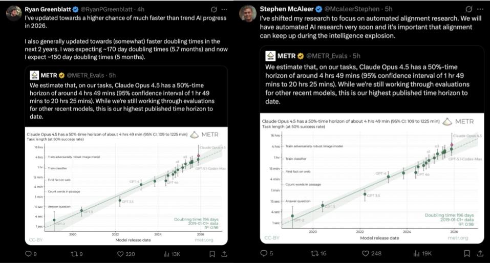
This doesn’t contradict common sense if you remember that Claude Opus 4.5 has a 50%-time horizon of around 4 hours 49 minutes (95% confidence interval: 1 hour 49 minutes to 20 hours 25 minutes).
Just think about it: from 1 hour 49 minutes up to 20 hours 25 minutes.
There simply isn’t enough data for reliable conclusions.
Lower R^2 is a natural consequence of the x axis being shorter, in an experimental setup with both signal and noise. In the extreme, imagine that we only benchmarked models on 47 minute tasks. AIs will naturally do better at some 47 minute tasks than others. Since R^2 is variance explained by the correlation with x, and x is always 47 minutes, all the variance in task success rate will be due to other factors and the R^2 will be zero.
In fact this is why we constructed SWAA—to increase the R^2 in worlds where the trend is real. In a world where models were not actually better at tasks with shorter human time, the R^2 would be lower when you add more data, so it’s a very scientifically normal thing to do.
Thanks for writing this. I disagree with some of the claims in this post but, as one of the authors on the original paper, I’ve been meaning to write a post on ways time horizon is overrated/misinterpreted. Limited number and distribution of tasks is definitely near the top of the list.
edit: posted!
I also applaud the effort to interrogate the underlying data. I have also been dismayed at people hanging dramatic updates off (what usually should be?) 1-few bits of surprisal. (I don’t think METR can be fairly blamed for others ~hunting noise in the ‘last’ datapoint—the CIs are clearly printed on the graph.)
Per other comments, I think the more theoretical worries in the OP miss the mark: you should end up with something like logistic curve if task length is unbounded but success probability is (0, 1); logging does a fairly good job at linearizing the data (although at least for sonnet 3.7 the fit collapses in the 2hr+ region, and eyeballing the other histograms suggests this might generalize).
Yet I think they may be in right neighbourhood of a ‘construct validity’ worry around time horizons. In precis (hopefully a full post someday):
Unlike (e.g.) ‘how fast can you run?’ or ‘how much can you lift?’ there’s seldom a handy cardinal scale for intellectual performance: IQ = 0 does not mean ‘zero intelligence’, nor you having double my chess ELO means you are twice as good at chess as I am. (Even if you’re happy not having a meaningful zero, meaningful interval scales don’t exist either.)
Besides issues of general overprediction, it seems hard to tell how meaningful a D increment on X benchmark is. The function from ‘benchmark score’ to ‘irl importance’ (or ‘AI capabilities’) could be almost anything monotonic: from “any nonzero score is a cataclysmic breakthrough (but any further increment matters little on the margin”, to “long march through the ‘nines’ (so all scores <99.9% are ~equally worthless), and everything in between.
Hence the utility of METR’s time horizons as a (/the only?) cardinal measure: ‘doubling’ is meaningful, and (if treated, as it often is—and I suspect more than METR would like it to be—as a proxy for ‘AI capabilities in general’) it shows a broad trend of exponentially increasing capabilities over last few years. (+/- discourse over whether recent data points indicate even more dramatic acceleration, ‘hitting the wall’, etc.)
What is load-bearing for this account is the essentially exponential transformation between ‘raw’ scores on HCAST etc. to time horizons. Per OP (and comments), you can get a similar plot with just the raw scores, and it is largely the transformation from that to time horizons which gives (e.g.) Opus 4.5, scoring 75%, ~double the time horizon of GPT5 (70%), or ~treble the time horizon of o3 (66%). If the y-axis of the figure was instead “composite accuracy (SWAA+HCAST+REBench)”, the figure might be grist for the mill of folks like Gary Marcus: “A whole year of dramatically increasing investment and computation, and all it got you was another 10%.”
It goes without saying METR didn’t simply stipulate ’linear score improvement = exponentially increasing time horizons”: it arose from a lot of admirable empirical work demonstrating the human completion time is roughly log-distributed.
But at least when taken as the colloquial byword for AI capabilities, this crucial contour feels a bit too mechanistic to me. I take that you can generalise the technique widely to other benchmarks deepens rather than alleviates this concern: if human benchmarking exercises would give log-distributed horizons across the items in many (/most?) benchmarks, such that progressive linear increments in model performance would give a finding of exponentially improving capabilities, maybe too much is being proven.
Taking the horizons (and their changes) literally has dubious face validity by my lights:
It doesn’t seem to me the frontier has gotten ~3x more capable over this year, and although I’m no software engineer, it doesn’t look from the outside like e.g. Opus 4.5 is 2x better at SWE than Opus 4.1, etc.
Presumably we could benchmark humans against the time horizons (IIRC not everyone used in the benchmarking could successfully complete the task), or at least the benchmarks from which time horizons could be imputed from. I’d at least be doubtful our best guess should be Alice (who cracks 75%) is 3x the SWE of Bob who hits 65%, etc.
That said, given our grasp of the ‘true cardinal scale of intellect’ is murky—or fictitious—even if my vibes are common, it looks reasonable to deny them rather than the facially contradicting data.
Perhaps the underlying moral of the jagged frontier is there isn’t some crisp (at least crisp + practically accessible) measure out there re. ‘general intelligence’ (or even general measures of intelligence when particularly applied: cf. ‘twice as good at chess’), and we should focus on metrics specific to whatever real-world impact we are interested in (maybe for ‘AI generally’, just trend extrapolate from ‘economy generally’?). But if the story of benchmarks over the last while is they are missing whatever intellectual dark matter intervenes between ‘benchmark assessing X’ and ‘actually Xing’, maybe you can’t derive sturdy synthetic y-axis yardsticks from their distorted timber: the transfer function from ‘time horizon’ to ‘irl importance’ is a similar value of ”??” as the original benchmarks were.
Not sure I agree with this, we constructed the benchmark to span a wide range, and the empirical work was mostly to show that the model success rate curve was logistic in human time.
This isn’t always the case. What matters for a benchmark is a range that spans many orders of magnitude, not exactly log distribution, and in that report, we saw that many benchmarks generally spanned narrower ranges than the METR task suite, so there isn’t enough data to prove that increments in model performance. In others, task length was poorly correlated with difficulty for models. But taken together, the fact that models went from 0% to saturating MATH500, then the AIME, and now IMO points to a dramatic increase in capabilities.
I also think our everyday experience points to something like an exponential relationship between an intuitive “task complexity rating” and human time. It’s natural to think of a level n+1 task as being decomposable into several level n tasks (eg get groceries = drive to the store, shop, drive back from the store) which naturally gives you exponential.
Some of this is probably the benchmark being unrepresentative of real tasks, but it’s not clear why an agent with 2x the time horizon should feel 2x better. When using an assistant with double the time horizon on real tasks, you need to intervene half as much, but each intervention takes you longer, since it’s written about double the code, fails in more complicated ways, and you have less understanding of what it’s doing. Combined with Amdahl’s law effects, I wouldn’t be surprised if doubling the time horizon only causes a speedup of 1.2x or so on average on tasks much longer than the agent’s time horizon, which are still most of them.
No, whether it continues the log-linear trend depends on WHEN a new model solves one additional task.
Using the logistic function to fit task success probability vs task length is not load-bearing for the time horizon computation.
If the task lengths in the data set were uniformly distributed (in log-space) you could just take the overall accuracy and look up the task length of that percentile in the data and that would be nearly identical to the 50% horizon. This would replace the logistic assumption with a step-function assumption, but because the logistic is point symmetric in the 50% point, it’s roughly the same value.
Put differently: There is an interval where the model goes from basically 100% to basically 0% and the logistic just takes the point in the middle for the 50% horizon. And there are many other methods that also take the point in the middle (possibly in a less robust way, but that would just make the trend a little more noisy).
I think your feeling that this is suspect comes more from the choice of the log-space not the choice of the fitting function. It feels a bit circular to say “we gonna assume that the log-space of task length is the natural way to look at model competence” and then get the result that through linear time model competence improves linearly in that log-space. I think it is also rather this choice of log-space not of the logistic that is motivated by the log-linear plot of model success rate vs human time to complete.
Also I would point out that the validity of the time horizons computed for the current models is not just based on these 16 tasks, but on the preceding six year trend + replications of exponential trends in other datasets. It’s great to point out that current measurements have a ton of noise and are very gameable, but it’s hard to attack the conclusion of exponential progress in time horizons.
Okay but the six year trend is not super indicative of the future trend given the way the AI industry has developed in the last couple years. It would be much more useful to have a good measure of the recent trend, and it’s clear we don’t really have that. The wide uncertainty bounds already should have made it clear how noisy this result was, but people have tended to ignore the range and put a lot of stock in the point estimate. The log linear trend may well be legit (probably is) but the use of just 14 tasks to fit the key portion of the results is absurd.
We also need to challenge the assumption that a task that is hard for humans is equally hard for AI, and vice versa — that is, that there exists a strong correlation between human difficulty and AI difficulty.
Consider a simple analogy. Suppose we want to determine the time horizon of a calculator on multiplication tasks. Let one number have n digits and the other have m digits (in base 10). For a human, the complexity is O(n⋅m).
A calculator, however, will successfully solve all such tasks as long as they do not cause overflow, because its success does not correlate with computational complexity in the human sense, but rather with the number of digits in the result.
This illustrates that human task difficulty and AI task difficulty can be fundamentally misaligned.
Strong-upvoted for picking more well-justified holes in that graph I contributed to. See also my post on this topic for some qualitative reasons to take that study with a grain of salt ( . . . as well as some debunked & redacted quantitative slander on my part, which this post reassures me happened to eventually be directionally correct, eto_bleh.gif).
Horizon length makes no sense fundamentally. The 9s of reliability don’t matter for anything but driving a car. Software and hacking and science and engineering are not a series of sequential steps. It is more like adding stuff to your house. If you can make a tiny improvement then you are net-helpful and you can build a cathedral. If you make improvements more often than you cause problems, anything is possible. If you break stuff more often than you fix it, then nothing is possible. It is a binary question. If you make big improvements, then small mistakes don’t matter. If you mess up stuff bigtime and can’t fix it, then big improvements are useless.
To clarify my point, I’m saying
A. Standalone/unattended (!) AI agents are clearly much worse than nothing, for both writing code (with a goal chosen in advance) and hacking (a prechosen target), they will clearly only mess up your plans.
If you want to build whatever or hack whoever, and you don’t care what, that’s a different story.
B. If your AI can make productive incremental progress, without messing up old code, writing false notes, citing misleading evidence, breaking infra, alerting the target, falsifying or ruining the tests, fooling the judge, etc, etc, then you can scale that to do basically anything. If you can lay a brick then you can make a cathedral.
If your whole fancy best-of-n-with-rollbacks system is able to lay down bricks, that also counts as OK.
C. I’m betting against the amazing-do-it-all-at-once-from-scratch AI being either a serious risk vector or driver of economic progress.
At least, if you do take over the world on Tuesday morning, it only counts as a victory if you don’t also accidentally give it all back on Tuesday afternoon.
D. I do think these task executions measure something meaningful, and are valuable to conduct, and we should try to extrapolate, but “task horizon length” is definitely not the thing to focus on here. Maybe something like the “zero fatal mistake” rate and the “net-forward-progress geometric mean” or something.
The world just does not look like “task horizons”. The world is made up of steps forward and steps backwards. A scientist or a CEO or an engineer or a horse or a door is measured by how many steps forward it brings you, per step backwards it takes you (which you weren’t able to spot and avoid obviously).
Fwdperbkwd is harder to measure than task horizons, maybe twice as hard, but not four times harder.
The strongest way I could put the punchline here is that I think AI agents will be useless until their code helps more than it hurts, then AI agents will replace coders completely. And you can only measure this by comparing agentless vs agentful approaches to the same task maybe (hey! METR did that too!)
And more ai-live-assistant is-it-worse-than-nothing-or-not experiments would be highly informative in my opinion!
If I want to know what level of task complexity I can give an LLM to get a guaranteed correct answer, horizon length is a good measure.
One particular chart in this post would be much easier to look at if it didn’t have an uncanny abomination wrapped in human skin stapled to it.
Perhaps humans generating training data are, for longer tasks, taking cognitive steps which are opaque to these models, or at least relatively more difficult to learn?
I’d wager 1:1 that this sort of abstraction-domain mismatch between human training data and LLMs is causing more of the HCAST weirdness than skewed finetuning investment.
That’s quite possible. I’m not sure how much that plays out with reinforcement learning training though.