SAE reconstruction errors are (empirically) pathological

[wesg]

Summary

Sparse Autoencoder (SAE) errors are empirically pathological: when a reconstructed activation vector is distance $ϵ$ from the original activation vector, substituting a randomly chosen point at the same distance changes the next token prediction probabilities significantly less than substituting the SAE reconstruction^[1] (measured by both KL and loss). This is true for all layers of the model (~2x to ~4.5x increase in KL and loss over baseline) and is not caused by feature suppression/​shrinkage. Assuming others replicate, these results suggest the proxy reconstruction objective is behaving pathologically. I am not sure why these errors occur but expect understanding this gap will give us deeper insight into SAEs while also providing an additional metric to guide methodological progress.

Introduction

As the interpretability community allocates more resources and increases reliance on SAEs, it is important to understand the limitation and potential flaws of this method.

SAEs are designed to find a sparse overcomplete feature basis for a model’s latent space. This is done by minimizing the joint reconstruction error of the input data and the L1 norm of the intermediate activations (to promote sparsity):

$$\underset{SAE}{min}\parallel x-SAE\left(x\right){\parallel }_2^2+\lambda \parallel SAE\left(x\right){\parallel }_1.$$

However, the true goal is to find a faithful feature decomposition that accurately captures the true causal variables in the model, and reconstruction error and sparsity are only easy-to-optimize proxy objectives. This begs the questions: how good of a proxy objective is this? Do the reconstructed representations faithfully preserve other model behavior? How much are we proxy gaming?

Naively, this training objective defines faithfulness as L2. But, another natural property of a “faithful” reconstruction is that substituting the original activation with the reconstruction should approximately preserve the next-token prediction probabilities. More formally, for a set of tokens $T$ and a model $M$, let $P=M\left(T\right)$ be the model’s true next token probabilities. Then let $Q_{SAE}=M\left(T|do\right(x\leftarrow SAE\left(x\right)\left)\right)$ be the next token probabilities after intervening on the model by replacing a particular activation $x$ (e.g. a residual stream state or a layer of MLP activations) with the SAE reconstruction of $x$. The more faithful the reconstruction, the lower the KL divergence between $P$ and $Q$ (denoted as $D_{KL}\left(P||Q_{SAE}\right)$) should be.

In this post, I study how $D_{KL}\left(P||Q_{SAE}\right)$ compares to several natural baselines based on random perturbations of the activation vectors $x$ which preserve some error property of the SAE construction (e.g., having the same $l_2$ reconstruction error or cosine similarity). I find that the KL divergence is significantly higher (2.2x − 4.5x) for the residual stream SAE reconstruction compared to the random perturbations and moderately higher (0.9x-1.7x) for attention out SAEs. This suggests that the SAE reconstruction is not faithful by our definition, as it does not preserve the next token prediction probabilities.

This observation is important because it suggests that SAEs make systematic, rather than random, errors and that continuing to drive down reconstruction error may not actually increase SAE faithfulness. This potentially indicates that current SAEs are missing out on important parts of the learned representations of the model. The good news is that this KL-gap presents a clear target for methodological improvement and a new metric for evaluating SAEs. I intend to explore this in future work.

Intuition: how big a deal is this (KL) difference?

For some intuition, here are several real examples of the top-25 output token probabilities at the end of a prompt when patching in SAE and $ϵ$-random reconstructions compared to the original model’s next-token distribution (note the use of log-probabilities and the KL in the legend).

For additional intuition on KL divergence, see this excellent post.

Experiments and Results

I conduct most of my experiments on Joseph Bloom’s GPT2-small residual stream SAEs with 32x expansion factor on 2 million tokens (16k sequences of length 128). I also replicate the basic results on these Attention SAEs.

My code can be found in this branch of a fork of Joseph’s library.

Intervention Types

To evaluate the faithfulness of the SAE reconstruction, I consider several types of interventions. Assume that $x$ is the original activation vector and $x_{SAE}$ is the SAE reconstruction of $x$.

• $ϵ$-random substitution: $x_{ϵ}$ is a random vector with $\parallel x_{ϵ}-x{\parallel }_2=\parallel x_{SAE}-x{\parallel }_2=ϵ$. I.e., both $x_{SAE}$ and $x_{ϵ}$ are random vectors on the $ϵ$-ball around $x$.

• $\theta$-random substitution: $x_{\theta }$ is a random vector with $\cos (x_{\theta },x)=\cos (x_{SAE},x)=\cos \left(\theta \right)$. I consider both versions where the norm of $x_{\theta }$ is adjusted to be $\parallel x\parallel$ and $\parallel x_{SAE}\parallel$.

• SAE-norm substitution: this is the same as the original activation vector except the norm is altered to the SAE norm $x^{\prime }=(\parallel x_{SAE}\parallel /\parallel x\parallel )\ast x$. This is a baseline to isolate the effect of the norm change from the SAE reconstruction, a known pathology identified here.

• norm-corrected SAE substitution: this is the same as $x_{SAE}$ except the norm is altered to the true norm $x_{SAE}^{\prime }=(\parallel x\parallel /\parallel x_{SAE}\parallel )\ast x_{SAE}$. Similar motivation as above.

In addition to these different kinds of perturbations, I also consider applying the perturbations to 1) all tokens in the context 2) just a single token. This is to test the hypothesis that the pathology is caused by compounding and correlated errors (since the $ϵ$-random substitution errors are uncorrelated).

Here is are the average KL differences (across 2M tokens) for each intervention when intervened across all tokens in the context:

There are 3 clusters of error magnitudes:

• The $x_{SAE}$ and norm-corrected $x_{SAE}$ are both high with norm-corrected slightly higher (this makes sense because it has a higher L2 reconstruction error).

• $ϵ$-random and both variants of $\theta$-random have much lower but non-trivial KL compared to the SAE reconstruction. They are all about the same because random vectors in a high dimensional space are almost-surely almost-orthogonal so the $ϵ$-random perturbation has an effect similar to the $\theta$-random perturbation.

• Most importantly, the SAE-norm substitution has an almost 0 KL divergence. This is important because it shows that the difference is not caused by the smaller norm (a known problem with SAEs) but the direction.

Given these observations, in the rest of the post I mostly focus on the $ϵ$-random substitution as the most natural baseline.

Layerwise Intervention Results in More Detail

Next, I consider distributional statistics to get a better sense for how the errors are distributed and how this distribution varies between layers.

This is a histogram of the KL differences for all layers under $ϵ$-random substitution and the SAE reconstruction (and since I clamp the tails at 1.0 for legibility, I also report the 99.9th percentile). Again the substitution happens for all tokens in the context (and again for a single layer at a time). Note the log scale.

Observe the whole distribution is shifted, rather than a few outliers driving the mean increase.

Here is the same plot but instead of KL divergence, I plot the cross-entropy loss difference (with mean instead of 99.9p). While KL measures deviation from the original distribution, the loss difference measures the degradation in the model’s ability to predict the true next token.

Just as with KL, the mean loss increase of the SAE substitution is 2-4x higher compared to the $ϵ$-random baseline.

Finally, here is a breakdown of the KL differences by position in the context.

Single Token Intervention Results

One possibility is that the KL divergence gap is driven by compounding errors which are correlated in the SAE substitutions but uncorrelated in the baselines (since the noise is isotropic). To test this, I consider the KL divergence when applying the substitution to a single token in the context.

In this experiment I intervene on token 32 in the context and measure the KL divergence for the next 16 tokens (averaged across 16,000 contexts). As before, there is a clear gap between the SAE and $ϵ$-random substitution, and this gap persists through the following tokens (although the magnitude of the effect depends on how early the layer is).

For clarity, here is the KL bar chart for just token 32 and the following token 33.

While the KL divergence of all interventions is lower overall for the single token intervention, the SAE substitution KL gap is preserved—it is still always >2x higher than the $ϵ$-random substitution KL for the present token and the following token (except token 33 layer 11).

How pathological are the errors?

To get additional intuition on how pathological the SAE errors are, I try randomly sampling many $ϵ$-random vectors for the same token, and compare the KL divergence of the SAE substitution to the distribution of $ϵ$-random substitutions.

Each subplot below depicts the KL divergence distribution for 500 $ϵ$-random vectors and the KL of the true SAE substitution for a single token at position 48 in the context. The substitution is only performed for this token and is performed on the layer 6 residual stream. Note the number of standard deviations from the $ϵ$-random mean labeled in the legend.

What I take from this plot is that the gap has pretty high variance. It is not the case that every SAE substitution is kind-of-bad, but rather there are both many SAE reconstructions that are around the expectation and many reconstructions that are very bad.

When do these errors happen?

Is there some pattern in when the KL gap is large? Previously I showed there to be some relationship with absolute position in the context. As expected, there is also a relationship with reconstruction cosine similarity (a larger error will create a larger gap, all things equal). Because SAE L0 is correlated with reconstruction cosine sim, there is also a small correlation with the number of active features.

However, the strongest correlations I could find were with respect to the KL gap of other layers.

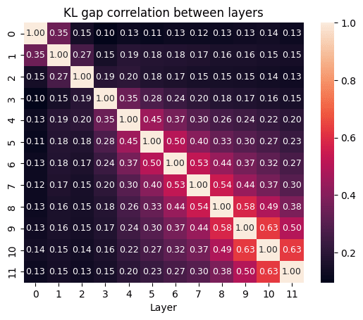
This suggests that some tokens are consistently more difficult for SAEs to faithfully represent. What are these tokens? These are the top 20 by average KL gap for layer 6 (and occur at least 5 times)

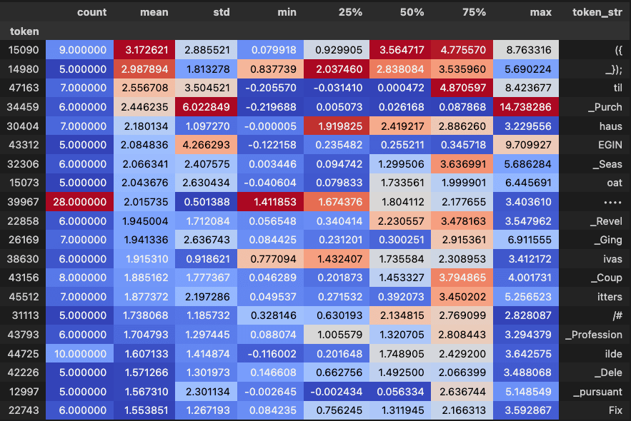
Beyond there not being an obvious pattern, notice the variance is quite high. I take this to mean the representational failures are more contextual. While these tokens seem rarer, there is no correlation between token frequency and KL gap.

For additional analysis on reconstruction failures, see this post.

Replication with Attention SAEs

Finally, I run a basic replication on SAEs trained on the concatenated z-vectors of the attention heads of GPT2-small.

While there is still a KL gap between the SAE and $ϵ$-random substitution, it is smaller (0.9x-1.7x) than the residual stream SAEs, and a larger fraction of the difference is due to the norm change (though it depends on the layer). This was expected since substituting the output of a single layer is a much smaller change than substituting the entire residual stream. Specifically, a residual stream SAE tries to reconstruct the sum of all previous layer outputs, and therefore replacing it is in effect replacing the entire history of the model, in contrast to just updating a single layer output.

Concluding Thoughts

Why is this happening?

I am still not sure yet! My very basic exploratory analysis did not turn up anything obvious. Here are a few hypotheses:

• $ϵ$-random is a bad baseline because activation space is not isotropic (or some other reason I do not understand) and this is not actually that unexpected or interesting. Consider a hypothetical 1000-dim activation space where most activations only lie in a 500-dim subspace and the model mostly ignores the other 500 dimensions (e.g. for robustness?). Then the random perturbation gets applied across all dimensions and the perturbation in the effective activation space is smaller leading to a smaller KL.

• Some features are dense (or groupwise dense, i.e., frequently co-occur together). Due to the L1 penalty, some of these dense features are not represented. However, for KL it ends up being better to nosily represent all the features than to accurately represent some fraction of them. For examples, consider:

  • [Dense] The position embedding matrix in GPT2-small is rank ~20. Therefore to accurately reconstruct absolute context position you already need 20 active features!

  • [Groupwise dense] Manifold features families where a continuous feature is represented by a finite feature discretization (e.g., curve detectors where multiple activate) or hierarchical feature families like space and time; E.g., the in_central_park feature is potentially a subtype of in_new_york_city, in_new_york_state, in_usa, etc. which might all activate at once; similar for a date-time which would require activating features at many temporal scales (in addition to adjacent points in the manifold). Perhaps such features are also learned in combinations.

• Some features are fundamentally nonlinear, and the SAE is having difficulty reconstructing these.

• Training FLOPs: perhaps these SAEs are undertrained. One test for this is checking if the KL gap gets better or worse with more training.

• Training recipe: each of these SAEs are trained to have approximately the same average L0 loss (average number of features) and have the same fan-out width. In practice, I expect that the number of active features and the number of in-principle representable features to vary throughout network depth. The large variability in KL gap by layer is suggestive.

• Quirk of GPT2: while I tested two different families of SAEs trained by two different groups, they were both on GPT2! I’d guess that other models behave differently (e.g. something like this might matter).

Takeaways

Assuming these findings replicate to other SAEs (please replicate on your own models!):

• SAEs empirically make non-random pathological errors. In particular, SAE reconstructions are consistently on a bad part of the $ϵ$-ball as measured by KL divergence and absolute loss increase.

• Both SAE KL and $ϵ$-random substitution KL divergence should be a standard SAE evaluation metric to measure faithfulness of the reconstruction.

  • Conceptually, loss recovered seems a worse metric than KL divergence. Faithful reconstructions should preserve all token probabilities, but loss only compares the probabilities for the true next token^[2].

• Closing the gap between SAE and $ϵ$-random substitution KL divergence is a promising direction for future work.

Future work

I intend to continue working in this direction. The three main work streams are

• Check that this replicates in other SAEs and that the $ϵ$-random baseline is actually sensible.

• Do a more thorough analysis of when and why these errors occur and test some of the aforementioned hypotheses.

• Develop SAE training methods which close the KL-gap.

Acknowledgements

I would like to thank Carl Guo, Janice Yang, Joseph Bloom, and Neel Nanda for feedback on this post. I am also grateful to be supported by an Openphil early career grant.

1. ^

   That is, substituting an SAE reconstructed vector $x_{SAE}$ for the original activation vector $x$ changes the model prediction much more than a random vector $x_{ϵ}$ where $\parallel x_{SAE}-x{\parallel }_2=\parallel x_{ϵ}-x{\parallel }_2=ϵ$.

2. ^

   E.g., consider the case where both the original model and the SAE substituted model have place probability $p$ on the correct token but their top token probabilities are all different. Loss recovered will imply that the reconstruction is perfect when it is actually quite bad.E.g., consider the case where both the original model and the SAE substituted model have place probability $p$ on the correct token but their top token probabilities are all different. Loss recovered will imply that the reconstruction is perfect when it is actually quite bad.

[jake_mendel]

I’m very unsure about this (have thought for less than 10 mins etc etc) but my first impression is that this is tentative evidence in favour of SAEs doing sensible things. In my model (outlined in our post on computation in superposition) the property of activation vectors that matters is their readoffs in different directions: the value of their dot product with various different directions in a readoff overbasis. Future computation takes the values of these readoffs as inputs, and it can only happen in superposition with an error correcting mechanism for dealing with interference, which may look like a threshold below which a readoff is treated as zero. When you add in a small random vector, it is almost-surely almost-orthogonal to all the readoff directions that are used in the future layers, so all the readoff values hardly change. Perhaps the change is within the scale that error correction deals with, so few readoffs change after noise filtering and the logits change by a small amount. However, if you add in a small vector that is aligned to the feature overbasis, then it will concentrate all its changes on a few features, which can lead to different computation happening and substantially different logits.

This story suggests that if you plot the KL difference as a function of position on a small hypersphere centered at the true activation vector (v computationally expensive), you will find spikes that are aligned with the feature directions. If SAEs are doing the sensible thing and approximately learning the true feature directions, then any small error in the SAE activations leads to a worse KL increase than you’d expect from a random pertubation of the activation vector.

The main reason I’m not that confident in this story (beyond uncertainty about whether I’m thinking in terms of the right concepts at all) is that this is what would happen if the SAEs learned perfect feature directions/​unembeddings (second layer of the SAE) but imperfect SAE activations/​embeddings. I’m less sure how to think about the type of errors you get when you are learning both the embed and unembed at the same time.

Here’s a prediction that would be further evidence that SAEs are behaving sensibly: add a small pertubation $\delta$ to the SAE activations in a way that preserves the L0, and call the perturbed SAE output $x_{SAE}^{\delta }$. This activation vector should get worse KL than $x_{SAE}+x_{\delta }$ (with random $x_{\delta }$ chosen such that $||x_{SAE}^{\delta }-x_{SAE}|{|}_2=||x_{\delta }|{|}_2$).

[wesg]

This is a great comment! The basic argument makes sense to me, though based on how much variability there is in this plot, I think the story is more complicated. Specifically, I think your theory predicts that the SAE reconstructed KL should always be out on the tail, and these random perturbations should have low variance in their effect on KL.

I will do some follow up experiments to test different versions of this story.

[tailcalled]

Could this be explained if SAEs only find a subset of the features so therefore the reconstructions are just entirely missing random features whereas random noise is just random and therefore mostly ignored?

[wesg]

Yup! I think something like this is probably going on. I blamed this on L1 but this could also be some other learning or architectural failure (eg, not enough capacity):

Some features are dense (or groupwise dense, i.e., frequently co-occur together). Due to the L1 penalty, some of these dense features are not represented. However, for KL it ends up being better to nosily represent all the features than to accurately represent some fraction of them.

[Neel Nanda]

Great post! I’m pretty surprised by this result, and don’t have a clear story for what’s going on. Though my guess is closer to “adding noise with equal norm to the error is not a fair comparison, for some reason” than “SAEs are fundamentally broken”. I’d love to see someone try to figure out WTF is going on.

[Erik Jenner]

Nice post, would be great to understand what’s going on here!

Minor comment unrelated to your main points:

Conceptually, loss recovered seems a worse metric than KL divergence. Faithful reconstructions should preserve all token probabilities, but loss only compares the probabilities for the true next token

I don’t think it’s clear we want SAEs to be that faithful, for similar reasons as briefly mentioned here and in the comments of that post. The question is whether differences in the distribution are “interesting behavior” that we want to explain or whether we should think of them as basically random noise that we’re better off ignoring. If the unperturbed model assigns substantially higher probability to the correct token than after an SAE reconstruction, then it’s a good guess that this is “interesting behavior”. But if there are just differences on other random tokens, that seems less clear. That said, I’m kind of torn on this and do agree we might want to explain cases where the model is confidently wrong, and the SAE reconstruction significantly changes the way it’s wrong.

[wesg]

Yes this a good consideration. I think

1. KL as a metric makes a good tradeoff here by mostly ignoring changes to tokens the original model treated as low probability (as opposed to measuring something more cursed like log prob L2 distance) and so I think captures the more interesting differences.

2. This motivates having good baselines to determine what this noise floor should be.

[Gunnar_Zarncke]

I have difficulty following all of these metrics without being able to relate them to the “concepts” being represented and measured. You say:

What I take from this plot is that the gap has pretty high variance. It is not the case that every SAE substitution is kind-of-bad, but rather there are both many SAE reconstructions that are around the expectation and many reconstructions that are very bad.

But it is hard to judge what is a high variance and whether the bad reconstructions are so because of systematic error or insufficient stability of the model or something else.

The only thing that helps me get an intuition about the concepts is the table with the top 20 tokens by average KL gap. These tokens seem rare? I think it is plausible that the model doesn’t “know” much about them and that might lead to the larger errors? It’s hard to say without more information what tokens representing what concepts are affected.

[wesg]

This was also my hypothesis when I first looked at the table. However, I think this is mostly an illusion. The sample means for rare tokens will have very high standard errors and so it is the case that rare tokens will have both unusually high average KL gap and unusually negative average KL gap mostly. And indeed, the correlation between token frequency and KL gap is approximately 0.

[Christopher James Hart]

$ϵ$-random is a bad baseline because activation space is not isotropic (or some other reason I do not understand) and this is not actually that unexpected or interesting.

Isn’t this just the answer? To rephrase:

The SAE is only able to represent a subset of the possible directions from the initial space when you force it to compress the space down.

If you take a magnitude from a direction where change matters, and then apply the magnitude to random dimensions most of which the model throws away, it will result in a smaller change.

[Logan Riggs]

I’ve only done replications on the mlp_out & attn_out for layers 0 & 1 for gpt2 small & pythia-70M

I chose same cos-sim instead of epsilon perturbations. My KL divergence is log plot, because one KL is ~2.6 for random perturbations.

I’m getting different results for GPT-2 attn_out Layer 0. My random perturbation is very large KL. This was replicated last week when I was checking how robust GPT2 vs Pythia is to perturbations in input (picture below). I think both results are actually correct, but my perturbation is for a low cos-sim (which if you see below shoots up for very small cos-sim diff). This is further substantiated by my SAE KL divergence for that layer being 0.46 which is larger than the SAE you show.

Your main results were on the residual stream, so I can try to replicate there next.

For my perturbation graph:

I add noise to change the cos-sim, but keep the norm at around 0.9 (which is similar to my SAE’s). GPT2 layer 0 attn_out really is an outlier in non-robustness compared to other layers. The results here show that different layers have different levels of robustness to noise for downstream CE loss. Combining w/​ your results, it would be nice to add points for the SAE’s cos-sim/​CE.

An alternative hypothesis to yours is that SAE’s outperform random perturbation at lower cos-sim, but suck at higher-cos-sim (which we care more about).

[Benjamin Wright]

One explanation for pathological errors is feature suppression/​feature shrinkage (link). I’d be interested to see if errors are still pathological even if you use the methodology I proposed for finetuning to fix shrinkage. Your method of fixing the norm of the input is close but not quite the same.

[wesg]

Right, I suppose there could be two reasons scale finetuning works

1. The L1 penalty reduces the norm of the reconstruction, but does so proportionally across all active features so a ~uniform boost in scale can mostly fix the reconstruction

2. Due to activation magnitude or frequency or something else, features are inconsistently suppressed and therefore need to be scaled in the correct proportion.

The SAE-norm patch baseline tests (1) but based on your results, the scale factors vary within 1-2x so seems more likely your improvements come more from (2).

I don’t see your code but you could test this easily by evaluating your SAEs with this hook.

[Aidan Ewart]

Edit: As per @Logan Riggs’s comment, I seem to have misunderstood what was being meant by ‘loss recovered’, so this comment is not relevant.

Cool post! However, it feels a little early to conclude that

> Conceptually, loss recovered seems a worse metric than KL divergence.

In toy settings (i.e. trying to apply SAEs to a standard sparse coding setting where we know the ground truth factors, like in https://​​www.lesswrong.com/​​posts/​​z6QQJbtpkEAX3Aojj/​​interim-research-report-taking-features-out-of-superposition/​​ ), SAEs do not acheive zero reconstruction loss even when they recover the ground truth overbasis with high mean max cosine similarity (and the situation is even worse when noise is present). It’s never seemed that obvious to me that we should be aiming to have SAE reconstruction loss go to zero as we train better SAEs, as we could plausibly still use the basis that the SAEs extract, without having to plug the SAE into a ‘production’ system for mech interp (in which case, we would want good reconstructions).

[Logan Riggs]

Seems tangential. I interpreted loss recovered is CE-related (not reconstruction related).