Addressing Feature Suppression in SAEs
Produced as part of the ML Alignment Theory Scholars Program—Winter 2023-24 Cohort as part of Lee Sharkey’s stream.
TL;DR
Sparse autoencoders are a method of resolving superposition by recovering linearly encoded “features” inside activations. Unfortunately, despite the great recent success of SAEs at extracting human interpretable features, they fail to perfectly reconstruct the activations. For instance, Cunningham et al. (2023) note that replacing the residual stream of layer 2 of Pythia-70m with the reconstructed output of an SAE increased the perplexity of the model on the Pile from 25 to 40. It is important for interpretability that the features we extract accurately represent what the model is doing.
In this post, I show how and why SAEs have a reconstruction gap due to ‘feature suppression’. Then, I look at a few ways to fix this while maintaining SAEs interpretability. By modifying and fine-tuning a pre-trained SAE, we achieve a decrease in mean square error and a reduction in the perplexity increase upon patching activations into the LLM.
Finally, I compare a theoretical example to the observed amounts of feature suppression in Pythia 70m, showing that features are suppressed based on both the strength of their activations and their frequency of activation.
Feature Suppression
The architecture of an SAE is:
The loss function usually combines a MSE reconstruction loss with a sparsity term, like , where is the dimension of . When training the SAE on this loss, the decoder’s weight matrix is fixed to have unit norm for each feature (column).
The reason for feature suppression is simple: The training loss has two terms, only one of which is reconstruction. Therefore, reconstruction isn’t perfect. In particular, the loss function pushes for smaller values, leading to suppressed features and worse reconstruction.
An illustrative example of feature suppression
As an example, consider the trivial case where there is only one binary feature in one dimension. That is, with probability and otherwise. Then, ideally the optimal SAE would extract feature activations of and have a decoder with .
However, if we were to train an SAE optimizing the loss function , we get a different result. If we ignore bias terms for simplicity of argument, and say that the encoder outputs feature activation if and otherwise, then the optimization problem becomes:
Therefore the feature is scaled by a factor of compared to optimal. This is an example of feature suppression.
If we allow the ground truth feature to have an activation strength upon activation and dimension , this factor becomes:
In other words, instead of having the ground truth activation , the SAE learns an activation of , a constant amount less. Features with activation strengths below would be completely killed off by the SAE.
Feature suppression is a significant problem in current SAEs
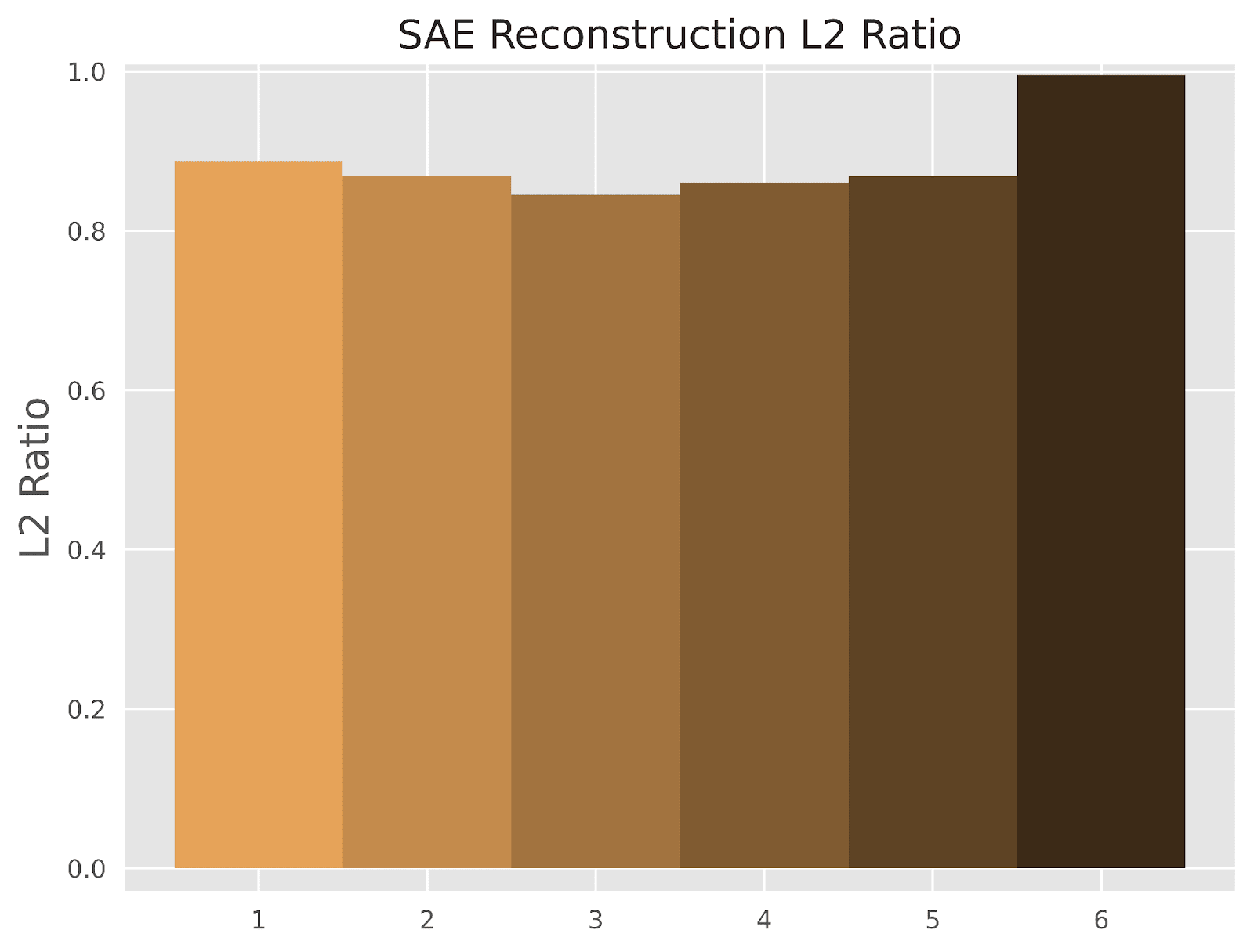
To experimentally verify that feature suppression affects SAEs, we first trained SAEs on the residual stream output of each layer of Pythia-70m with an L1 sparsity penalty (coefficient 2e-3) on 6 epochs of 100 million tokens of OpenWebText, with batch size 64 and learning rate 1e-3, resulting in roughly 13-80 feature activations per token. The residual stream of Pythia-70m had a dimension size of 512 and we used a dictionary size of 2048, for a four times scale up.
If feature suppression had a noticeable effect, we’d see that the SAE reconstructions had noticeably smaller L2 norms than the inputs. Therefore, the expected ratio of the norms (or “L2 Ratio”) can be a proxy for measuring the presence of feature suppression. Indeed, Figure 1 shows feature suppression to be significant, with all but the last layer showing that the reconstructions are less than the norm of the activations on average.
How can we fix feature suppression in trained SAEs?
Here we evaluate a few different methods to fix the problem of feature suppression. The general approach will be to take a normally-trained SAE and then fine-tune a subset of its parameters without the presence of a sparsity penalty. Freezing parts of the SAE is imperative to prevent degradation of the sparse structure of learned features.
We first slightly modify the SAE by introducing an element-wise scaling factor for each feature in-between the encoder and decoder, represented as the vector :
In our experiments, we permit different sets of parameters to train, labeled by a method name as laid out in Table 1.
| Method Name | Trainable Parameters |
| Scale | |
| Decoder | |
| Unrotated Decoder | |
| Encoder | |
| Unrotated Encoder | |
| Unrotated All |
Table 1: The trainable parameters of each fine-tuning method.
We also include a “Baseline” method which is simply training the original SAE without any changes to architecture or loss function on the same number of tokens. We expect there to be no change in the “baseline” method if the SAE is already trained to convergence.
We fine-tuned the SAEs using each of these methods on the same 100 million token subset of OpenWebText and made no change to other hyperparameters. Most of these methods (except for the “Encoder” method) converged by 20-30 million tokens, which is much faster than the SAE pretraining. As a caveat, it may be worth training for longer than is strictly necessary for convergence if you wish to analyze how extremely rare features are modified by fine-tuning.
Fine-tuning Reduces Feature Suppression
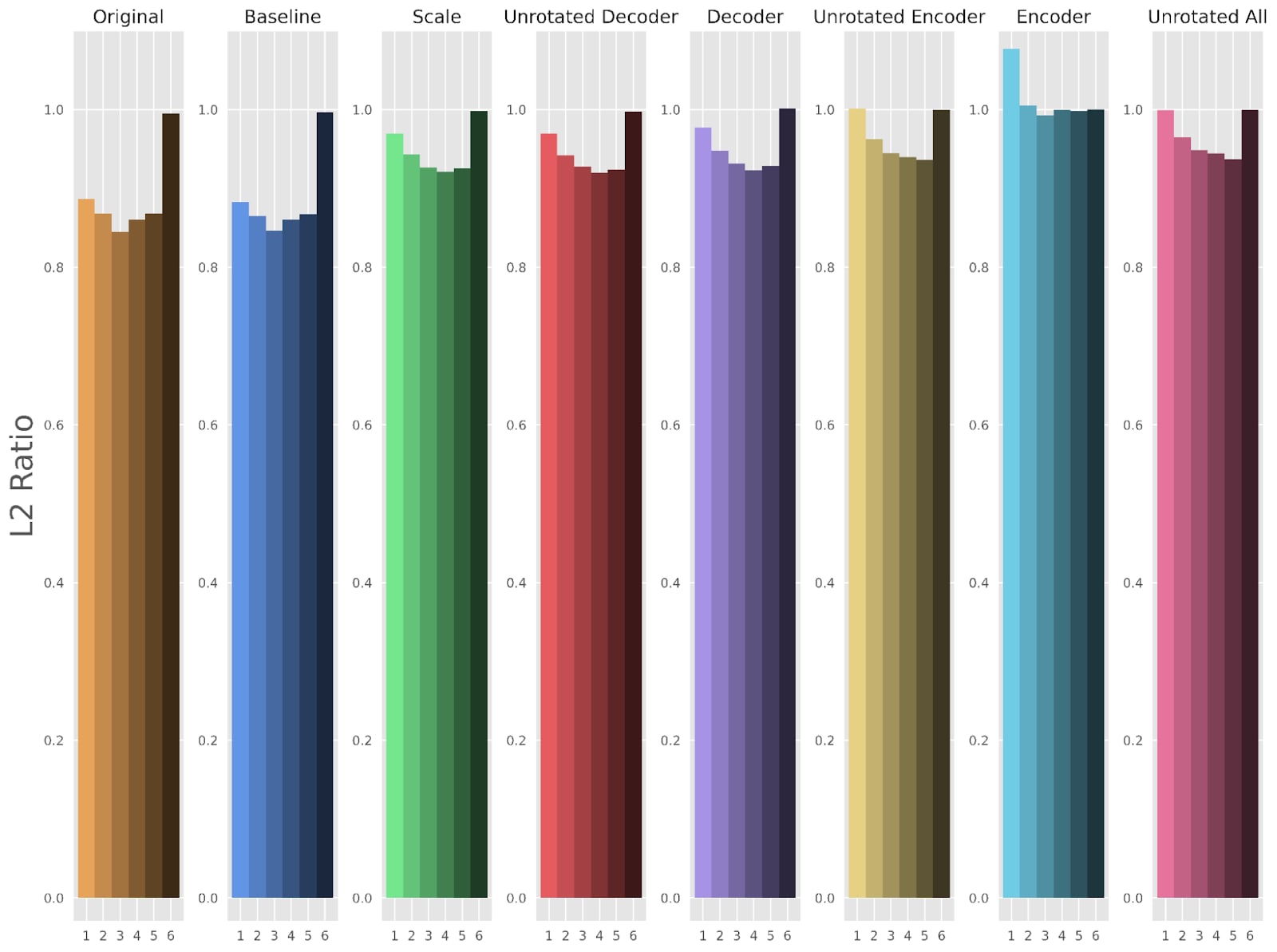
The first thing that stands out about these different fine-tuning approaches was that any method that fine-tuned the encoder led to a drastic reduction in sparsity (Figure 2). This is clearly undesirable, so in future plots we omit methods that fine-tune the encoder (but full versions of the plots are available in the appendix).
We next show that the “Scale”, “Decoder”, and “Unrotated Decoder” methods address the feature suppression issue in Figure 3, which expands Figure 1 to plot the L2 ratio for our other methods. Each fine-tuning method greatly improves the L2 ratio to be closer to , as desired, although there is still some gap left in layers 1 through 5. This may be due to missing features in the encoder and other errors that cannot be recovered in the decoder.

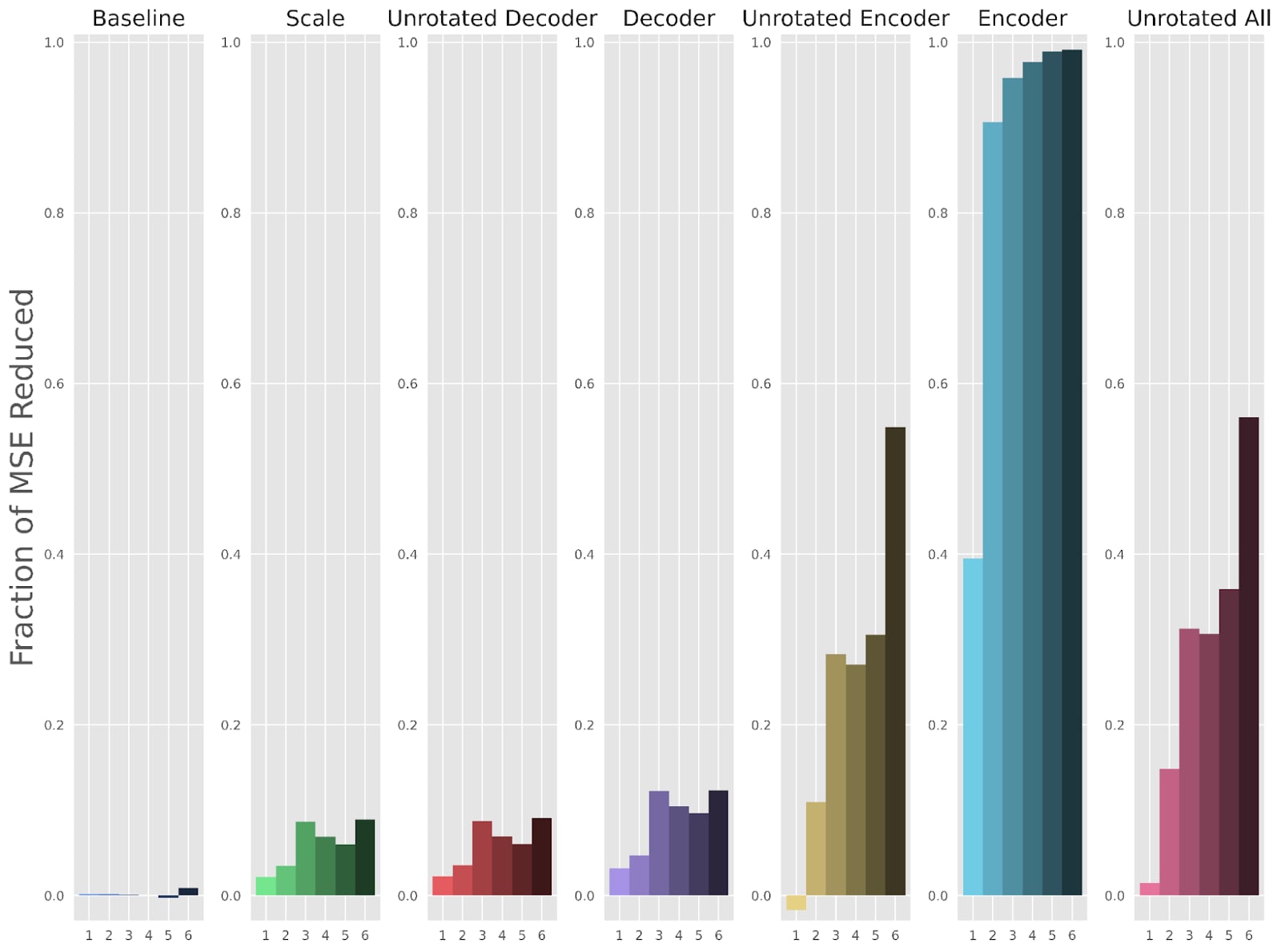
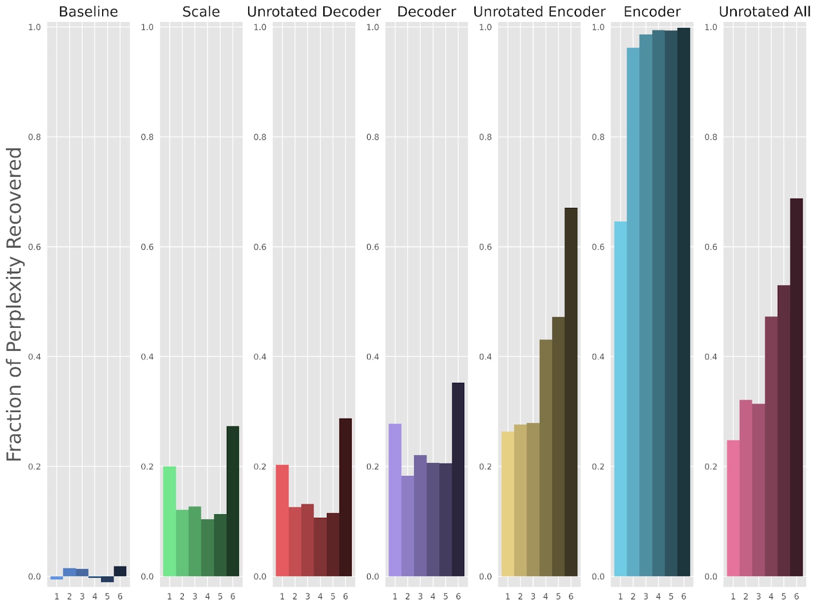
Next, we examine how well our fine-tuning methods improve upon the reconstruction loss and the perplexity of the LLM after patching in the activation reconstruction. Figures 4 and 5 use a fractional scale, where a 1 means the fine-tuned SAE has completely recovered the original LLM’s performance, and a 0 means the fine-tuned SAE has done just as poorly as the original SAE.
The “Decoder” method reduces reconstruction loss MSE by (Figure 4) and the perplexity gap by (Figure 5). MSE and perplexity values in addition to other metrics for each individual layer are also included in the appendix.
Activation Strength Causes Feature Suppression
In this section we analyze how our fine-tuning methods address feature suppression. We look from the lens of feature activation frequency and activation strength.
Taking a look at a graph of empirical feature frequencies in Figure 6, we immediately see an almost discontinuous jump in activation frequencies in the middle for all but the last layer, which has a slightly more gradual change. We found that the features on the infrequent side of the jump were essentially dead features with no significant change upon fine-tuning, and therefore we exclude them from future plots. We also note that the graph looks mostly similar if instead of plotting feature frequencies we plotted the sum of activation values across the dataset.
We focus the rest of our analysis on layer 5, but the results are similar for other layers.
A theoretical example predicts frequency isn’t a factor
Our illustrative example predicted that the frequency of a feature’s activation, , would be independent from the amount that feature gets suppressed in a trained SAE. This is because, in the single binary feature scenario, an SAE would learn activation values according to:
This formula does not include . Therefore, when adding new features to the theoretical example, as long as each feature has sufficiently small interference with every other feature, an SAE will treat each feature independently and similarly to the single feature scenario.
Moreover, activation strength is a factor when considering the multiplicative scaling factor, , but not when taking the difference between SAE activation strength and ground truth strength .
Fine-tuning does not fix regression dilution
While our illustrative example didn’t show much of a relationship with frequency, there is a separate way in which frequency can cause features to be poorly represented by an SAE, which is regression dilution:
Feature suppression is when the sparsity term in the loss function induces smaller feature activations.
Regression dilution is the effect where adding noise to an input of a linear regression results in a decreased learned coefficient. This effect is not based on any sparsity term in the loss function.
We believe the frequency by which a feature activates may have a relationship with regression dilution, because of interference with other features in the encoder. The rarer a feature is, the more likely any activation of that feature is due to accidental interference from nearby features. This results in the learned SAE feature being noisy, and therefore regression dilution results in a lower feature activation.
Because regression dilution is an artifact of the encoder, it is not something that our decoder-based fine-tuning methods can fix. Therefore, we still predict no relationship between frequency and empirically observed feature scaling upon fine-tuning.
Experimental measurements agree for activation strength, disagree for frequency
Our illustrative example from earlier predicted that scaling after fine-tuning anti-correlates with activation strength and is independent from frequency; while Figure 7 supports the trend for activation strength, it also shows that frequency is not independent. The correlation between and was , while the correlation between and was , contrary to predictions.
Even when isolating the impact of frequency or activation strength, the other variable still had a large magnitude of correlation with scaling. The partial correlations were and for and , respectively.
Meanwhile, the illustrative example also predicted that the impact of average activation strength vanishes when we consider the average change in activation strength instead of the learned scaling factor, and the experimental results mostly agree, as plotted in Figure 8. Then, the correlations between , and became -, respectively, showing that activation strength has significantly reduced in importance. The partial correlations also became and .
Conclusion
In conclusion, training with a sparsity penalty leads to suppression of features, predominantly features with frequent but weak activations. By inserting a scaling factor and fine-tuning the decoder without the sparsity penalty, we can achieve a improvement in reconstruction loss and a recovery of perplexity without changing when features activate. Even with nothing but a scaling factor, which in theory means interpretability should be unaffected, fine-tuning can achieve a improvement in reconstruction loss and a recovery of perplexity.
This work suggests that if we want to insert our SAEs into our models and use their outputs in the forward pass of the model (which we might want to do to study the effects of different features on model internals and outputs), then we should consider fine-tuning the scale of the learned features post-SAE-training, or we should identify some other way to reduce feature suppression.
Appendix
Related Work
Feature suppression is similar to what happens in the Lasso method of linear regression, where there is a L1 penalty on the weights in addition to the squared error reconstruction loss. Lasso stands for “Least Absolute Shrinkage and Selection Operator”; as its name says, Lasso regression tends to both select a sparse set of the input dimensions to use, as well as shrink the usage of those inputs. This effect is well-known, and besides choosing different sparsity penalties, one proposal is retraining the linear regression without Lasso after Lasso selects a sparse set of parameters (Belloni and Chernozhukov, 2009). This approach mirrors our approach to mitigating feature suppression in SAEs.
Lee et al., 2019 also point out how freezing parts of a language model during fine-tuning can be a good idea, which is similar to our motivation for keeping the encoder frozen while fine-tuning SAEs.
Extended Data
We show the full version of Figures 3, 4, and 5, including the methods that allowed parts of the encoder to train.
Summary Statistics for SAEs
| Layer | SAE MSE | Fine-tuned MSE | SAE Perplexity | Fine-tuned Perplexity | SAE L0 | Fine-tuned L0 | SAE L2 Ratio | Fine-tuned L2 Ratio | Dead Features |
| 1 | 0.0159 | 0.0154 | 93.84 | 78.77 | 13.34 | 13.34 | 0.88651067 | 0.9771778 | 101 |
| 2 | 0.0270 | 0.0257 | 76.21 | 69.53 | 16.80 | 16.80 | 0.86834979 | 0.9477061 | 112 |
| 3 | 0.0431 | 0.0379 | 85.29 | 75.22 | 45.52 | 45.52 | 0.84479147 | 0.93124998 | 422 |
| 4 | 0.0507 | 0.0454 | 85.11 | 75.72 | 38.53 | 38.53 | 0.86063075 | 0.92301691 | 248 |
| 5 | 0.0645 | 0.0582 | 67.58 | 61.83 | 49.78 | 49.78 | 0.86816871 | 0.92854148 | 72 |
| 6 | 0.1167 | 0.1024 | 73.16 | 61.33 | 80.66 | 80.66 | 0.9951911 | 1.00137651 | 6 |
Table A1: Metrics for the base SAEs and the fine-tuned SAEs under the “Decoder” method. “L0” measures the average number of feature activations per token, and “L2 Ratio” measures the average ratio of the norm of the output to the norm of the input. “Dead Features” shows how many of the 2048 features never activate on the dataset.
Low strength/high frequency features also rotate more
We measure the cosine similarity between the decoder dictionary vector before and after fine-tuning. Future work could examine what causes rotations in more detail.
- Mech interp is not pre-paradigmatic by (10 Jun 2025 13:39 UTC; 213 points)
- Efficient Dictionary Learning with Switch Sparse Autoencoders by (22 Jul 2024 18:45 UTC; 118 points)
- SAE reconstruction errors are (empirically) pathological by (29 Mar 2024 16:37 UTC; 108 points)
- Sparsify: A mechanistic interpretability research agenda by (3 Apr 2024 12:34 UTC; 97 points)
- Apollo Research 1-year update by (29 May 2024 17:44 UTC; 93 points)
- [Full Post] Progress Update #1 from the GDM Mech Interp Team by (19 Apr 2024 19:06 UTC; 80 points)
- ProLU: A Nonlinearity for Sparse Autoencoders by (23 Apr 2024 14:09 UTC; 44 points)
- Evaluating Sparse Autoencoders with Board Game Models by (2 Aug 2024 19:50 UTC; 38 points)
- Normalizing Sparse Autoencoders by (8 Apr 2024 6:17 UTC; 22 points)
- Research Report: Alternative sparsity methods for sparse autoencoders with OthelloGPT. by (14 Jun 2024 0:57 UTC; 17 points)
- An Introduction to SAEs and their Variants for Mech Interp by (19 Apr 2025 14:09 UTC; 17 points)
- 's comment on SAE reconstruction errors are (empirically) pathological by (29 Mar 2024 17:20 UTC; 2 points)
Awesome work! I’d be quite interested to know whether the benefits from this technique are equivalently significant with a larger SAE and also what the original perplexity was (when looking at the summary statistics table). I’ll probably reimplement at some point.
Also, kudos on the visualizations. Really love the color scales!
The original perplexity of the LLM was ~38 on the open web text slice I used. Thanks for the compliments!
Hey, I was wondering if you are using any weight decay during the training of the SAE? It feels to me that, being equivalent to implicit L2 minimization, this could also be the culprit. And if you don’t, how come the first layer doesn’t collapse to 0 while the second layer grows to infinity?
Thanks if you take the time to answer :)
Hi, thanks for your work. I was wondering why we use scaling to modify the activation here rather than using an analytical solution by compensating for the −cd/2 term.
Thanks for your amazing work! Theoretically I think that layers with higher input norms should have lower SAE L2 ratios, as they corresponds to higher feature activations that are penalized heavier. I wonder if your data confirms this hypothesis.