Probably you won’t be able to perform a data-driven habit stacking for self-improvement
Suppose you’re not happy with the quality of your sleep. You’ve already stopped doing the obviously harmful things (no more coffee at night), and your sleep has improved—but you’d like to work on it further. A coworker gives you an herbal mix with St. John’s wort and lavender. You try drinking it at night instead of coffee, and it does seem that sometimes your sleep really does get deeper than before. But sometimes it doesn’t. You’re willing to experiment, but how do you actually check whether the herbs work, or whether it’s just random variation?
Or suppose you’re not particularly satisfied with your productivity at work. Following the advice from “Atomic Habits” and books on workflow organization, you’ve introduced a few useful micro‑habits and ergonomic improvements. But what do you do once the low‑hanging fruits are picked up? Time is limited—you can’t implement everything that someone somewhere calls “useful”. Some habits are even mutually exclusive: it’s impossible to both socialize during lunch and sit alone in silence at the same time.
Or, for example, you want to achieve better results in fishing… you get the idea.
“Don’t underestimate the power of small things taken in large numbers” is a wise thought—but how do you figure out which small things actually work in your specific case? This is quite a roadblock on the path to becoming stronger. If you’ve taken a statistics course or have heard the term “A/B testing,” you probably already have a rough outline of an answer. Pick a target metric, collect historical data, then collect data after the chosen intervention, compare the average values before and after—and voilà, a scientifically grounded answer. The problem is that if you jump into a project like this without a solid plan, you’ll likely end up with a pile of useless numbers in a spreadsheet. Why this kind of endeavor is not for the faint‑hearted is exactly what I want to talk about in this article.
TLDR: Most effects you’re likely to encounter are too weak to detect against the background noise of everyday life. Even for a relatively noticeable effect, you need a carefully thought‑out experimental design and several months of work.
Notation
The following notation is used throughout the text:
D—variance (a measure of how spread out a random variable is)
For simplicity, the text below assumes that the intervention does not change the shape of the distribution (i.e. d is measured in units of
Minimal background for people who want to read the article but don’t know probability theory
Skip this section if you know what the symbols above mean and remember the basic properties of the normal distribution.
There will be no detailed derivations or rigorous proofs here. The article is far too short for me to teach even an introductory statistics course. But here’s a short summary so that readers unfamiliar with statistics can still follow the reasoning that comes next.
Imagine a regular six‑sided die. If it’s a fair die, the probability of rolling any given face is 1⁄6 = 16.66%. This is a uniform distribution—all outcomes are equally likely. It can be visualized with the following histogram:
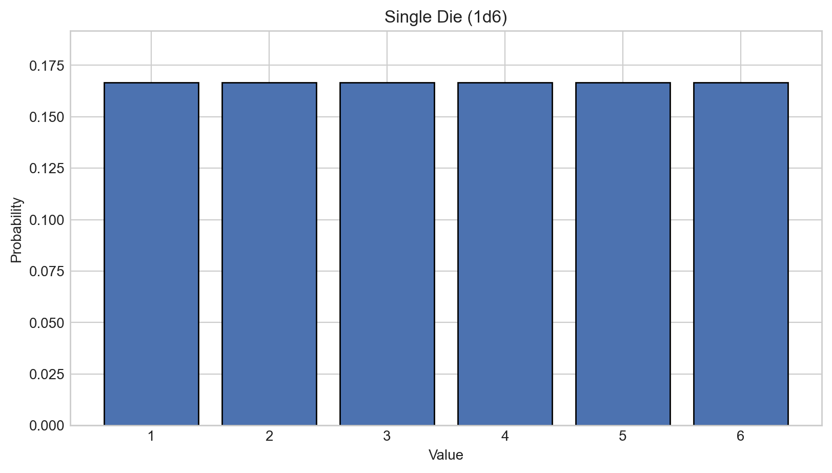
The horizontal axis shows the outcomes, the vertical axis shows their probabilities. The sum of probabilities over all outcomes is equal to one (100%).
But if we roll two six‑sided dice, the distribution of the sum of the outcomes is no longer uniform. If we list all possible outcomes:
1 + 1 = 2
1 + 2 = 3
2 + 1 = 3
1 + 3 = 4
2 + 2 = 4
3 + 1 = 4
1 + 4 = 5
...
5 + 6 = 11
6 + 5 = 11
6 + 6 = 12
we can see that 2 can only occur if both dice show 1 (which happens in 1 out of 36 cases). A sum of 3 can happen in two ways: the first die is 1 and the second is 2, or vice versa—so the probability is 2⁄36. The chance of rolling a 4 is even higher: 3⁄36, and so on. The largest number of combinations produce a sum of 7. These include cases where both dice land near the middle of the range (3+4, 4+3), as well as cases where a small value is compensated by a large one (1+6, 2+5, 5+2, 6+1).
The bars of the histogram form a triangle. What happens if we roll three six‑sided dice instead?
You can see that the center becomes smoother, while the tails spread out. Again, this happens because getting a 3 or an 18 requires all three dice to land on 1 or 6 respectively. Central values, on the other hand, can arise both when all dice land near the middle and when small values compensate large ones.
If we take 25 dice, the resulting plot takes a particular bell shape:
For practical purposes, a curve like this is already quite close to a normal distribution. Many things in our lives follow an (approximately) normal distribution: the height of men of a fixed age in a given country, measurement errors of most instruments, your mood over the course of a year. This happens for the same reason as with the sum of dice. You’re in a good mood when everything goes according to plan (all dice roll 5–6). You’re in a bad mood when nothing works out (all dice roll 1–2). But an average mood can result both from an unremarkable day and from good things compensating for bad ones.
(“Didn’t get enough sleep this night. But I remembered my favorite school teacher in the morning, which gave me a motivational boost. Then there was a traffic jam on the way to work—so irritating! At least the day is sunny; you can feel that spring is coming—I love spring.”)
Probability theory says that the elements being summed don’t have to be uniformly distributed. As long as they have a sufficiently “nice” shape, their sum will converge to a normal distribution. This is called the central limit theorem. And “niceness” holds surprisingly often.
The bell curve can have different widths, and we’d like to be able to measure this spread. Simply measuring the distance between the leftmost and rightmost values is impractical, because values near the edges of the bell occur very rarely. So in practice, we use variance (
The red arrows in the picture show distances from the center to several points. To compute the standard deviation, we take all these distances, square each of them, sum them up, divide by their count, and then take the square root of the result.
It is known that 68% of elements of a normal distribution lie within the range
Now suppose we have two sets of values: an original random distribution and the same distribution shifted by some amount. For example, a database of how well students performed on a test after 48 weeks of studying a subject, and how well they performed after 96 weeks. How do we estimate how much doubling the time improves the results? It’s convenient to measure this shift in units of
What if the intervention not only shifts the mean, but also increases the spread of values? That’s not a problem—we take the average
This is called Cohen’s d statistic. Scientific papers usually report results using exactly this measure.
How large of effects should you expect from self‑experimentation?
It’s hard to answer this question in general. Some people are trying to optimize sleep quality, others are aiming to gain muscles. Let’s calibrate expectations—here are Cohen’s d values for a few well‑studied effects:
Taking creatine (a dietary supplement widely used among bodybuilders), depending on the protocol and how outcomes are measured, yields an additional performance gain of about d = 0.27–0.59[1].
Strength training with a coach, as opposed to training alone, adds another d = 0.28–0.4 depending on how performance is measured[2].
Meta‑analyses estimate the average effect of antidepressants at around d = 0.3[3]. The effect is smaller in cases of mild depression. In real life, however, one should expect a much larger impact: a doctor can try several medications and fine‑tune the dosage.
There is no consensus on the effectiveness of mindfulness meditation for treating anxiety disorders. Studies show a wide spread of results, but an average estimate of d = 0.2 seems quite plausible[4][5].
Moderate‑intensity strength training (60–80% of one‑rep max) reduces glycated hemoglobin levels by about d = 0.4[6].
Additional financial education classes yield d = 0.15 for financial knowledge (test scores) and d = 0.07 for financially responsible behavior (for example, building a larger emergency fund)[7].
On the one hand, your personal life situation or biochemistry might amplify effects that are useless for most people. On top of that, studies are limited by the fact that the same “dose” of an intervention is applied to all participants, whereas you can fine‑tune the “dose” much more precisely for yourself. On the other hand, you’re unlikely to test anything on yourself that’s stronger than prescription antidepressants. Also, most likely you’ll want to optimize things like “mood” or “energy throughout the day.” It’s rare for something to simultaneously affect biology, externally imposed daily schedules, psychology, and the habits feeding into these metrics. So expecting effects of d > 1 from any intervention in these cases would be strange. Either you already know about such interventions and are already doing them (you’ve almost certainly gone to school—not some specific course, but school in general). Or you know about them but aren’t doing them for good reasons (moving to a Buddhist monastery would almost certainly have a strong effect on anxiety but there are legitimate reasons not to do that). Or these are major life‑changing decisions that don’t just happen casually, and that are hard to reproduce and study—leaving an abusive partner, or radically changing career track.
As a result, in my opinion, if you’re trying to optimize your life by tweaking habits and selecting supplements, you’re effectively “hunting” for effects in the range d = 0.1–0.4.
What does d = 0.1–0.4 actually mean in real life?
The 10th percentile of electric motor assemblers in the US earns about $25k per year, while the 90th percentile earns $56.5k[9]. Roughly speaking, the standard deviation of this distribution is around $8.5k per year, and 0.2 of that is $1.7k per year. That’s enough to buy a decent bicycle in Texas.
If someone has between 5 and 45 free hours per week for leisure in 95% of cases, then an effect that increases free time by
If in 95% of cases you read 40–160 pages per week (a 400‑page book per month), then
In medical literature, effects of
Sounds tempting—but then what’s the catch?
How many observations, exactly?
To estimate the absolute effect of an intervention, we take a set of observations before the intervention and another set after it, and then compare the mean values of the two sets. The problem is that we need a lot of data. For example, in the figure below we have only 4 observations—and we got unlucky. Even though the green distribution is actually to the right of the blue one, based on our limited data we would have to conclude that it’s to the left, and by quite a lot:
(There’s a similar issue when estimating the standard deviation needed to compute Cohen’s d, but let’s focus on the means for now.) All we can hope for is that with more observations, the chance of getting unlucky with all of them decreases. For example, here some of the variability partially cancels out:
Computing the mean difference for the plot above gives
The pooled standard deviation, computed using the method from the previous section, is equal to 1, so the d‑value is also 0.6:
So how many observations do we actually need to be confident? Let’s look at how well the estimated value converges to the true effect. Below are plots from twenty simulations showing how our estimate of the difference between two normal distributions with D = 1 depends on the number of observations. We’re trying to detect true effects of d = 0.1, d = 0.2, and d = 0.3, respectively:
From these plots we can draw several conclusions:
On average, we do converge to the true effect. The more observations we have, the closer we get.
That said, you don’t know in advance which simulation branch you’re on. You can either underestimate or overestimate the effect of the intervention.
The spread of the estimates shrinks relatively quickly at first, but after about 200 observations, adding more data barely reduces the spread. At the given noise level, it takes around 1200 observations for the simulation curves to consistently fall within a
The convergence rate depends only very weakly on the true effect size.
This isn’t visible in the plots, but the single most important factor is the noise level—the natural variability of the observed quantity.
If you look closely at the plots, you’ll see that even for an effect of d = 0.3, you need more than 175 observations before all simulation runs at least register a positive effect. For d = 0.1, you need roughly 1000. But even this understates how hard the experiment really is! In practice, we need to distinguish between interventions that have an effect and interventions that have no effect at all. That means the bundles of simulations for “effect” and “no effect” need to be sufficiently separated for us to tell which bundle our observed line belongs to:
From the image above, it’s clear that separating these bundles requires around 600–700 observations.
The plots are intuitive, but not very formal. What does theory say?
p‑value
In science, the standard way to assess whether we can reject the null hypothesis (no effect; the intervention has no impact) is via a p‑value test. The p‑value for an effect is the probability that the null hypothesis is true and that we observe a difference between two datasets that is at least as large as the one we got. Conventionally, if this probability is below 5%, we reject the null hypothesis. This is the well‑known criterion
How can we estimate the probability of observing the measured difference if there is actually no effect? Once again, the normal distribution comes to the rescue. The sum and the difference of normally distributed random variables are themselves normally distributed[12]. As a result, the difference of sample means
Below are plots showing how confidence in our conclusion grows with the number of observations, corresponding to the convergence plots above. The bold line shows the average across the p‑value experiments above. This is not exactly the true expected p‑value curve, but it already makes the point: achieving 95% confidence requires a lot of observations.
So what should we expect theoretically? We can “invert” the derivation above and compute how much data is needed to detect, with a given probability, an effect of known size d. Here are a few scenarios:
Theory says that to have 5% false positives and 5% false negatives, we need:
For d = 0.3 - about 580 observations (i.e. roughly 290 before the intervention and 290 after; note how well this matches the separation point of the d‑value bundles above)
For d = 0.2 - about 1300 observations
For d = 0.1 - about 5200 (!) observations
If we lower the bar slightly and allow 5% false positives and 20% false negatives, we need:
For d = 0.3 - about 350 observations
For d = 0.2 - about 800 observations
For d = 0.1 - about 3150 observations
If we lower the bar even further and allow 20% false positives and 20% false negatives:
d = 0.3 − 200 observations
d = 0.2 − 250 observations
d = 0.1 − 1800 observations
And finally, if we are absolutely certain that the effect must be positive and use a one‑sided test:
d = 0.3 − 126 observations
d = 0.2 − 280 observations
d = 0.1 − 1120 observations
So even if we significantly relax the confidence requirements and completely ignore the possibility that the intervention could do harm instead of good, detecting a not‑so‑weak effect of d = 0.3 still requires four months of observations! As a reminder, this is roughly the effect size of the first correctly chosen antidepressant for a patient with moderate depression. You can basically give up on trying to measure anything weaker. Vitamins (if you don’t have a specific deficiency), fish oil, and an extra 20 minutes of walking during the day (unless you’re usually completely sedentary) simply won’t be visible—even with very careful tracking.
Additional complications
But that’s still not all. There are several more effects worth paying attention to—each of them further increases the number of observations required.
Non‑linear interactions
It’s very rare for an intervention’s effect to be linear across the entire range we care about. Most interventions have a saturation threshold. The first extra hour of walking gives a larger effect than the third. This isn’t too bad, although it does mean we tend to underestimate the effect of partial interventions.
Much worse is when an intervention’s effect looks like an inverted U. The first cup of coffee makes you more alert, while the fifth makes you shake in hyper‑focused anxiety. Less than six hours of sleep is bad, but more than ten hours of sleep is also bad. Catching the optimal level of exposure is not always easy. Ideally, you’d want to test several intensity levels—which means running the experiment at least twice.
Accumulation and time‑to‑effect
Many interventions don’t produce an immediate effect. For example, atomoxetine (a medication for ADHD) has an effect ranging from d = 0.4 up to d = 2 (!) depending on the patient group and how symptoms are measured[15], but it can take up to four weeks to accumulate in the body. As a result, some ADHD patients may abandon even such an effective drug before it has time to work. The results of going to the gym or starting psychotherapy take even longer to show up.
Often, it’s not even clear what delay to expect. If you’re studying the relationship between weight loss and back pain, you probably shouldn’t expect the pain to go away immediately after losing weight. The damage to the back has already been done—it needs time to heal. But how long it takes for the effect to reach a plateau is unclear.
Side conditions and seasonality
The same intervention can be useful at one time and useless at another. Seasonality is the most obvious factor here, but it’s not the only one. An extra hour of walking or a vitamin D capsule may have a stronger effect in winter than in summer, because people tend to get less light and physical activity during the cold months. Sports supplements may work when you’re in a caloric surplus and do nothing in a deficit. Meditation might improve mood in the morning but harm sleep quality in the evening.
Substitution effects
Suppose you want to study how sleep deprivation affects you. You collect data on work productivity depending on whether you slept 6 or 8 hours. But if, after a six‑hour night, you drink more tea—and tea has a stimulating effect on you—you might not see any productivity drop from sleep deprivation in the data at all. You either need to fix all other parameters of the system (hard to do in practice), or collect data on them as well. Accounting for substitution effects complicates the model. And it’s often unclear in advance which factors might act as substitutes.
“Noisy” measurement units
If you’re measuring your own happiness or energy levels, you’ll run into consistency issues. People can usually distinguish between feeling 2⁄10 and 8⁄10 - but those extreme states don’t happen very often. Most of the time, you need to tell apart 4⁄10 from 5⁄10 and 5⁄10 from 6⁄10, and not everyone is that good at introspection. By the second month of a study, people get tired of doing this and start choosing between 4 and 5 at random. If there are no systematic biases, the estimate should still eventually converge to the “true” value. Still, measurement error adds on top of the error in the underlying state, increasing overall noise—and with it, the required number of measurements.
You should try to ground abstract target metrics either in questionnaires or in objective physiological indicators. But filling out questionnaires takes time, and it requires willpower not to start answering them carelessly. Objective physiological metrics have a different problem: thanks to wearable devices they’re easy to collect, but they’re usually only very indirectly related to what you actually care about. You can use resting heart‑rate variability as a proxy for energy or anxiety levels—but the connection is quite indirect.
The observer effect
It’s hard to run a blind experiment when you’re both the researcher and the subject. This only really works for pills—and even then, not everyone is willing to deal with the organizational hassle. You know what effect you’re hoping for, and you’ll subconsciously nudge your ratings in the desired direction.
Moreover, the very act of monitoring changes the system. Data collection makes you engage with everything more consciously. Mindfulness is generally a good thing, but it also creates a gap between the experimental setup and real life. Checklists add friction to activities that used to be automatic. Excessive attention to your own happiness and calmness can itself cause depression and anxiety. This effect persists even if you know about it.
The general noise of life
Work deadlines, unexpected trips, illnesses, and periods of unusually good mood will create “holes” in your data. You’ll need to decide which data points “count,” or else log everything. You also need to decide what to do with missing data.
The best thing you can do for measurement quality is to reduce the overall noise level of the metric. Unfortunately, it’s very hard to put yourself into sufficiently controlled conditions for several months just to finish an experiment. You can try measuring more frequently, but beyond a certain (often unknown) threshold, increasing measurement frequency just collects more noise.
Conclusion and silver lining
“Data‑driven habit optimization” sounds cool and scientific, but in practice it’s a very situational endeavor. It’s worth attempting only if you:
are confident that the intervention you’re studying has at least d = 0.3 (see the list of effects above; do you really expect your intervention to be comparable?)
can come up with ways to deal with the additional complications described in the previous section
are ready to dedicate several months to the study
Estimate the expected cost of the data for such interventions. How much would you value information about the effect size? What is the expected cost of running the experiment? Even if this comparison suggests the study is worth doing, don’t expect an easy path or quick results. You will need this amount of dedication to the science.
EDIT: I would like to clarify in response to the comments that I don’t think that any data-driven life improvement is futile. My point that this particular flavor of rationalistic/nootrop-enthusiastic of searching and stacking d=0.1-0.3 improvements is very hard to implement. Other data-driven and generally goal-driven techniques are still very useful. For example:
As I’ve mentioned, you don’t know effect of certain intervention beforehand. In rare cases you may have a certain disorder you don’t know about and which can be greately ameliorated. If, say, you have vitamin A deficiency and when you start taking vitamin A supplements you notice effect. In this case it will be relatively easy to prove that effect is not a placebo.
So I guess, a fruitful strategy would be trying many things in sequence for a short period of time and investigating further if you notice any effect. Lossy but implementable.
Sometimes the mere noticing and paying attention what’s happening to you allows to you to thing if it’s worth changing your life in some aspects.
I’ve mentioned that sometimes the tracking itself introduces harmful friction into the process. However sometimes tracking itself helps! A common piece of advice in weightlifting is to track your progress. Same with losing weight.
It’s hard to fit outliers into normal distribution but noticing outliers in data motivates you to think why those outliers happened. They give you more information about yourself, uncover unknown unknowns.
Sometimes seeing negative patterns in data allows you to react to problems before they happen (on the other hand, see also: hypochondria)
Sometimes hard data help to gather your willpower to implement certain changes. For example when I do any intellectually demanding tasks after 22:00 my sleep quality drastically drops. I knew about that effect for some time but tried not to do anything at night only half-heartedly. Measuring that drop helped me to abstain from coding at night more consistently.
I’ve mentioned that it’s hard to achieve meaningful effect size on ‘happiness’ and other broad metrics but on the flip side it’s not that hard to achieve an effect on some narrow and easily measurable things. For example, tracking your blood sugar or blood pressure and expermenting on how different things affect them is much more reliable.
In rare cases experimenting triggers cascade effects or changes system around you enough that normal distribution is no longer applicable to modeling your situation.
- ^
- ^
- ^
- ^
- ^
- ^
- ^
- ^
- ^
- ^
- ^
- ^
Intuitively: if X is the result of summing N dice and Y is the result of summing M dice, then X+Y is the result of summing N+M dice—which only makes the distribution more bell‑shaped.
- ^
Intuition: imagine drawing pairs of numbers from the same set, one with your left hand and one with your right, and subtracting right from left. On average, for every pair ordered (first‑left, second‑right) there will be a corresponding (first‑right, second‑left). These opposite differences cancel out, and the mean ends up at zero.
- ^
When the
- ^
This article tries to argue the thesis “data driven self improvement isn’t able to be performed” and then argues why a particular approach to data driven self improvement is bad.
From November 2024 to the end of November 2025 I had a membership in a dance school and was going regularly. In Dezember 2025 is wasn’t going anymore and was moving less. Through the whole of Dezember my resilience values as measured by Oura were dropping and at Christmas I got very ill.
If I would have reacted sooner to the data it might have been quite good for my health. There wouldn’t have been any need to run a t-test. Just looking at the graph and taking it seriously would have been enough.
There was a time were lowest heart rate at night was normally in the 50 to 60 range. I don’t think I have done any large hikes in the decode before and was going to the birthday of a friend were we went hiking. In the next night my lowest heart rate was 45 (numbers from memory), this is a clear signal that something interesting was happening. No need to run a t-test.
When it comes to lifting weights, I think the leading advice is to track the data for your weight lifting. The point isn’t to run t-tests about the effects of creatine but to see whether you are improving at the lifting exercise you are doing and changing exercises if you don’t. That’s data driven self improvement.
There are a lot more dwarfs than the normal distribution would predict. There are some genetic mutations that have a relatively small effect on height and some that have a really big effect. If the people in your sample populations all have a bunch of genetic mutations that individually have a small effect you get something that looks like the normal distribution. If you however also have people with the mutations for dwarfism that have big effects, the distribution does not look like the normal distribution anymore.
I think if you are doing data driven self improvement, you do care about the outliers in data that are driven by the equivalent of the genetic mutation for dwarfism. If you just see them as noise, I don’t think that’s helpful.
Those are good points. Let me expand conclusion to clarify what I mean in my article and what I don’t mean—when data driven approach is helpful
I think you should retitle your post as well, it’s now misleading in light of all these counterexamples.
I had a persistent twitch in my face last year, and the cause was mysterious to me for many months and was giving me a lot of anxiety. I didn’t do any deliberate experimentation on it, but through natural variation in my behaviors and daily tracking of my data, I noticed that it was caused by a vitamin I was taking. It was a bit difficult to notice because the effect persisted beyond the days that I took the vitamin, and was further complicated because there were 3-4 other potential causes, some of which were actually correlated to my taking of the vitamin. But just seeing the data with natural variation over many months allowed me to make a change much quicker than I would have otherwise. And if I had been more deliberate about my methodology, it may have become a non-problem in the first place as I would’ve isolated a new substance’s effect before committing to taking it long-term.
Another anecdote: I know that staying up late and working on projects is a bad habit, but when I have a doubt about it and entertain a late-night working session, I can look at the actual data (even if subjective) and see that when I stay up past midnight, my quality of work goes down and I get a hit to my energy levels for 2-3 days following.
These are both examples where the effect on me was likely stronger than the 0.1-0.4 you mentioned. But how am I supposed to know what the effect size on me is in advance? Personal data tracking helps me identify cases where things I think are insignificant are actually significant (like taking specific vitamins) or where I know there is an effect, but do not have visibility into the full impact.
One more thing I want to mention is responder heterogeneity: Population level effect sizes can be weak, while individuals react strongly. While in expectation, you are going to be hunting for effect sizes of 0.1-0.4, in many cases (like antidepressants, creatine, supplements), if it works for you the individual response is much stronger and easier to detect.
This is a good point. I have very similar experience :) Let me edit conclusion section to clarify when data-driven approach is helpful.
While the comments provide a lot of counterexamples, I think the post still makes a very good point. I’ve done some self experimentation, see eg my melatonin self RCT, and I’m currently running a ~150 day experiment on several mood + productivity interventions in parallel, and I have to say, the power analysis beforehand is always disappointing. Even at 150 days, I’m basically biting the bullet of low statistical robustness of my findings, as I wasn’t willing to commit to doing this for a year or two. Additionally, this experiment can’t be blinded, so I can’t even be certain I’m measuring more than reporting bias (at least for some metrics). If I’m honest, I’m probably mostly doing it because I love data analysis and just look forward to that part. Ideally, I’ll get some insights out of it, but it’s unlikely they’ll be super surprising rather than just weak evidence roughly in the direction I already expect.
I once heard someone make the argument that self experimentation is worthwhile, but if you need statistical tools to evaluate it, then you’re doing it wrong, and you should rather look for effect sizes large enough that you easily and confidently notice them without calculating p-values. Seems like a valid claim to me. As long as there are high-variance things to try that may work amazingly well for you, it surely often makes sense to prioritize these rather than your average “this may improve my mood by 3%” intervention.
Indeed years ago I tried for several months to improve my poor sleep, varying and recording numerous variables from alcohol intake to timing of dinner and bed. Though I did a rather simple statistical analysis I was unable to identify anything that made a statistically significant difference—per your findings.
(In the end I did improve my sleep a lot—not due to my own experimentation but thanks to an excellent online course called Sleepio, clinically proven and prescribed by the NHS. Which identified something that hadn’t occurred to me—I was allowing too much time for sleep, ie setting my alarm too late, resulting in shallow sleep with too many night-time awakenings.)
I just skimmed but it does seem like the LessWrong bayes trope could help here. I practice if you’re trying to get data above random chance that’s unlikelt but if you have some intervrntions that are just on the edge of being worth it with an already strong prior, self experimentation cna help push it over the edge.