The Quantum Arena

[Eliezer Yudkowsky]

Previously in series: Classical Configuration Spaces

Yesterday, we looked at configuration spaces in classical physics. In classical physics, configuration spaces are a useful, but optional, point of view.

Today we look at quantum physics, which inherently takes place inside a configuration space, and cannot be taken out.

For a start, as you might guess, in quantum physics we deal with distributions of complex amplitudes, rather than probability distributions made up of positive real numbers. At left, I’ve used up 3 dimensions drawing a complex distribution over the position of one particle, A.

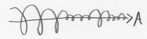
You may recall that yesterday, 3 dimensions let us display the position of two 1-dimensional particles plus the system evolution over time. Today, it’s taking us 3 dimensions just to visualize an amplitude distribution over the position of one 1-dimensional particle at a single moment in time. Which is why we did classical configuration spaces first.

To clarify the meaning of the above diagram, the left-to-right direction is the position of A.

The up-and-down direction, and the invisible third dimension that leaps out of the paper, are devoted to the complex amplitudes. Since a complex amplitude has a real and imaginary part, they use up 2 of our 3 dimensions.

Richard Feynman said to just imagine the complex amplitudes as little 2-dimensional arrows. This is as good a representation as any; little 2D arrows behave just the same way complex numbers do. (You add little arrows by starting at the origin, and moving along each arrow in sequence. You multiply little arrows by adding the angles and multiplying the lengths. This is isomorphic to the complex field.) So we can think of each position of the A particle as having a little arrow associated to it.

As you can see, the position of A bulges in two places—a big bulge to the left, and a smaller bulge at right. Way up at the level of classical observation, there would be a large probability (integrating over the squared modulus) of finding A somewhere to the left, and a smaller probability of finding it at the small bulge to the right.

Drawing a neat little graph of the A+B system would involve having a complex amplitude for each joint position of the A and B particles, which you could visualize as a hypersurface in 4 dimensions. I’d draw it for you, but I left my 4-dimensional pencil in the pocket of the 3rd leg of my other pants.

You may recall from yesterday that a plaid rectangular probability distribution factorizes into the product of two independent probability distributions.

This kind of independence-structure is one of several keys to recovering the illusion of individual particles from quantum amplitude distributions. If the amplitude distribution roughly factorizes, has subsystems A and B with Amplitude(X,Y) ~ Amplitude(X) * Amplitude(Y), then X and Y will seem to evolve roughly independently of each other.

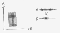
But maintaining the illusion of individuality is harder in quantum configuration spaces, because of the identity of particles. This identity cuts down the size of a 2-particle configuration space by ¹⁄₂, cuts down the size of a 3-particle configuration space by ¹⁄₆, and so on. Here, the diminished configuration space is shown for the 2-particle case:

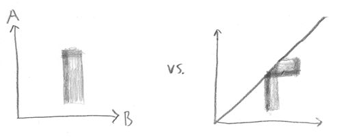
The quantum configuration space is over joint possibilities like “a particle here, a particle there”, not “this particle here, that particle there”. What would have been a neat little plaid pattern gets folded in on itself.

You might think that you could recover the structure by figuring out which particle is “really which”—i.e. if you see a “particle far forward, particle in middle”, you can guess that the first particle is A, and the second particle is B, because only A can be far forward; B just stays in the middle. (This configuration would lie in at the top of the original plaid pattern, the part that got folded over).

The problem with this is the little triangular region, where the folded plaid intersects itself. In this region, the folded-over amplitude distribution gets superposed, added together. Which makes an experimental difference, because the squared modulus of the sum is not the sum of the squared moduli.

In that little triangular region of quantum configuration space, there is simply no fact of the matter as to “which particle is which”. Actually, there never was any such fact; but there was an illusion of individuality, which in this case has broken down.

But even that isn’t the ultimate reason why you can’t take quantum physics out of configuration space.

In classical configuration spaces, you can take a single point in the configuration space, and the single point describes the entire state of a classical system. So you can take a single point in classical configuration space, and ask how the corresponding system develops over time. You can take a single point in classical configuration space, and ask, “Where does this one point go?”

The development over time of quantum systems depends on things like the second derivative of the amplitude distribution. Our laws of physics describe how amplitude distributions develop into new amplitude distributions. They do not describe, even in principle, how one configuration develops into another configuration.

(I pause to observe that physics books make it way, way, way too hard to figure out this extremely important fact. You’d think they’d tell you up front, “Hey, the evolution of a quantum system depends on stuff like the second derivative of the amplitude distribution, so you can’t possibly break it down into the evolution of individual configurations.” When I first saw the Schrödinger Equation it confused the hell out of me, because I thought the equation was supposed to apply to single configurations.)

If I’ve understood the laws of physics correctly, quantum mechanics still has an extremely important property of locality: You can determine the instantaneous change in the amplitude of a single configuration using only the infinitesimal neighborhood. If you forget that the space is continuous and think of it as a mesh of computer processors, each processor would only have to talk to its immediate neighbors to figure out what to do next. You do have to talk to your neighbors—but only your next-door neighbors, no telephone calls across town. (Technical term: “Markov neighborhood.”)

Conway’s Game of Life has the discrete version of this property; the future state of each cell depends only on its own state and the state of neighboring cells.

The second derivative—Laplacian, actually—is not a point property. But it is a local property, where knowing the immediate neighborhood tells you everything, regardless of what the rest of the distribution looks like. Potential energy, which also plays a role in the evolution of the amplitude, can be computed at a single positional configuration (if I’ve understood correctly).

There are mathematical transformations physicists use for their convenience, like viewing the system as an amplitude distribution over momenta rather than positions, which throw away this neighborhood structure (e.g. by making potential energy a non-locally-computable property). Well, mathematical convenience is a fine thing. But I strongly suspect that the physically real wavefunction has local dynamics. This kind of locality seems like an extremely important property, a candidate for something hardwired into the nature of reality and the structure of causation. Imposing locality is part of the jump from Newtonian mechanics to Special Relativity.

The temporal behavior of each amplitude in configuration space depends only on the amplitude at neighboring points. But you cannot figure out what happens to the amplitude of a point in quantum configuration space, by looking only at that one point. The future amplitude depends on the present second derivative of the amplitude distribution.

So you can’t say, as you can in classical physics, “If I had infinite knowledge about the system, all the particles would be in one definite position, and then I could figure out the exact future state of the system.”

If you had a point mass of amplitude, an infinitely sharp spike in the quantum arena, the amplitude distribution would not be twice differentiable and the future evolution of the system would be undefined. The known laws of physics would crumple up like tinfoil. Individual configurations don’t have quantum dynamics; amplitude distributions do.

A point mass of amplitude, concentrated into a single exact position in configuration space, does not correspond to a precisely known state of the universe. It is physical nonsense.

It’s like asking, in Conway’s Game of Life: “What is the future state of this one cell, regardless of the cells around it?” The immediate future of the cell depends on its immediate neighbors; its distant future may depend on distant neighbors.

Imagine trying to say, in a classical universe, “Well, we’ve got this probability distribution over this classical configuration space… but to find out where the system evolves, where the probability flows from each point, we’ve got to twice differentiate the probability distribution to figure out the dynamics.”

In classical physics, the position of a particle is a separate fact from its momentum. You can know exactly where a particle is, but not know exactly how fast it is moving.

In Conway’s Game of Life, the velocity of a glider is not a separate, additional fact about the board. Cells are only “alive” or “dead”, and the apparent motion of a glider arises from a configuration that repeats itself as the cell rules are applied. If you know the life/​death state of all the cells in a glider, you know the glider’s velocity; they are not separate facts.

In quantum physics, there’s an amplitude distribution over a configuration space of particle positions. Quantum dynamics specify how that amplitude distribution evolves over time. Maybe you start with a blob of amplitude centered over position X, and then a time T later, the amplitude distribution has evolved to have a similarly-shaped blob of amplitude at position X+D. Way up at the level of human researchers, this looks like a particle with velocity D/​T. But at the quantum level this behavior arises purely out of the amplitude distribution over positions, and the laws for how amplitude distributions evolve over time.

In quantum physics, if you know the exact current amplitude distribution over particle positions, you know the exact future behavior of the amplitude distribution. Ergo, you know how blobs of amplitude appear to propagate through the configuration space. Ergo, you know how fast the “particles” are “moving”. Full knowledge of the amplitude distribution over positions implies full knowledge of momenta.

Imagine trying to say, in a classical universe, “I twice differentiate the probability distribution over these particles’ positions, to physically determine how fast they’re going. So if I learned new information about where the particles were, they might end up moving at different speeds. If I got very precise information about where the particles were, this would physically cause the particles to start moving very fast, because the second derivative of probability would be very large.” Doesn’t sound all that sensible, does it? Don’t try to interpret this nonsense—it’s not even analogously correct. We’ll look at the horribly misnamed “Heisenberg Uncertainty Principle” later.

But that’s why you can’t take quantum physics out of configuration space. Individual configurations don’t have physics. Amplitude distributions have physics.

(Though you can regard the entire state of a quantum system—the whole amplitude distribution—as a single point in a space of infinite dimensionality: “Hilbert space.” But this is just a convenience of visualization. You imagine it in N dimensions, then let N go to infinity.)

Part of The Quantum Physics Sequence

Next post: “Feynman Paths”

Previous post: “Classical Configuration Spaces”

[JK]

Are point mass amplitudes really nonsense here? It’s common to view them as distributions, and then they can be differentiated like anything else. Is that not doable with Schrodinger’s equation?

[Psy-Kosh]

First, minor editing thingie: The bit at the top, that’s supposed to be a link to “classical configuration spaces” is just text, not a link.

Second, I think you’re wrong about “If you had a point mass of amplitude, an infinitely sharp spike in the quantum arena, the amplitude distribution would not be twice differentiable and the future evolution of the system would be undefined. The known laws of physics would crumple up like tinfoil. Individual configurations don’t have quantum dynamics; amplitude distributions do.”

Specifically, I do seem to remember learning how to deal with the time evolution of a dirac delta (constructed as the appropriate limit of a gaussian amplitude distribution). Basically (at least in non relativistic QM) it instantly flattens.

Also, I’m not entirely sure you’re completely right about amplitudes over positions in space being the actual physical reality underneath the math.

Specifically, wouldn’t relativity come in and say “eh? say what? positions in space? What do you mean?”

No prefered reference frame and all that. You could have them over configurations of stuff in spacetime, sure, but space itself? What one observer considers a single point at different times, a different observer will consider different points. (This obviously holds even in gallilean relativity) so I’d be very hesitant to claim that the amplitudes over configurations of positions in space has a deeper correspondence to the underlying reality than the various transforms that put the amplitudes over momentum space or whatever.

This bit was very helpful though: “This kind of independence-structure is one of several keys to recovering the illusion of individual particles from quantum amplitude distributions. If the amplitude distribution roughly factorizes, has subsystems A and B with Amplitude(X,Y) ~ Amplitude(X) * Amplitude(Y), then X and Y will seem to evolve roughly independently of each other.”

ie, a question that has kinda been bugging me is “well… then why does it look like amplitudes over configurations of ‘billiard balls’? why configurations of ‘billiard balls’ at all?” and that one bit helped be understand a little bit better where the billiard ball illusion is really coming from.

[Chris5]

They do not describe, even in principle, how one configuration develops into another configuration.

I’m going to just clarify this point, which I disagree with as written (not strictly wrong, but it overlooks something important). You can make a minor extension to quantum mechanics that does describe how one configuration develops into another. That extension is Bohmian mechanics, which is empirically equivalent to orthodox QM.

Basically, you postulate that in addition to the wavefunction, there is a configuration, and it obeys a certain law of motion which is guided by the wavefunction (the law is “switch to the hydrodynamic formulation change of variables, use the velocity law there”).

If you additionally postulate that the initial configuration is unknown, but randomly distributed like |psi(x)|^2 dx, you completely recover quantum mechanics. Among other things, you’ll never remove the initial uncertainty in a system governed by quantum mechanics.

So in fact, quantum mechanics is fully consistent with the existence of a single configuration.

However, that configuration alone doesn’t fully determine the future; you still need the wavefunction for that.

I’m not really one of the “true believers” (some folks fanatically love it), but I find it to be extremely helpful in developing intuition/​doing calculations. (Note: remove all hints of Bohmian mechanics before attempting to publish.)

[JessRiedel]

Psy-Kosh: In Quantum Field Theory, the fields (the analog of wavefunctions in non-relativistic Quantum Mechanics) evolve locally on the spacetime. This is given a precise, observer-independant (i.e. covariant) meaning. This property reduces to the spatially-local evolution of the wavefunction in QM which Eliezer is describing. Further, this indeed identifies position-space as “special”, compared to momentum-space or any other decomposition of the Hilbert space.

Eliezer: The wavefunctions in QM (and the fields in QFT) evolve locally under normal (Hermitian) evolution. However, Bell-type experiments show that wavefunction collapse is a non-local process (be it the preposterous Copenhagen-style collapse, or some flavor of decoherence). As far as I have read, the source of this non-locality is not understood.

[DanielLC]

I’m pretty sure Many Worlds doesn’t have waveform collapse. Also, I don’t think they’re talking about configuration space. They’re saying that particle a being in point A and particle b being in point B interacting is non-local. That configuration is one point, so it’s completely local.

[Roland2]

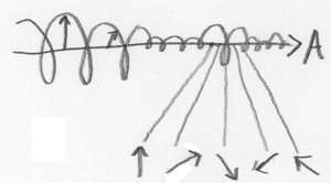
Regarding the top diagram:

Today, it’s taking us 3 dimensions just to visualize an amplitude distribution over the position of one 1-dimensional particle at a single moment in time.

To clarify the meaning of the above diagram, the left-to-right direction is the position of A.

Which of the following is true:

A) In the real universe there is a particle located in one specific position in that diagram. (In that case it is not clear to me what the amplitude distribution represents.)

OR

B) No particle exists in the real universe but all you have is an amplitude distribution over several positions giving the illusion that there is a particle in one position.

[JessRiedel]

Chris, in case you didn’t see me ask you last time...

http://​​www.overcomingbias.com/​​2008/​​04/​​philosophy-meet.html#comment-110472438

do you know of a good survey of decoherence?

[anonymous4]

Eliezer --

I’m loving this latest series of posts. I’m in the midst of exams right now, so I’ve only been able to skim them, but I will definitely go over them later. Keep up this important work!

• anonymous o.b. reader

[Toby_Ord2]

Eliezer,

Very minor quibble/​question. I assume you mean 2^Aleph_0 rather than Aleph_1. Unless one is doing something with the cardinals/​ordinals themselves, it is almost always the numbers Aleph_0, 2^Aleph_0, 2^2^Aleph_0… that come up rather than Aleph_n. You may therefore like the convenient Beth numbers instead, where:

Beth_0 = Aleph_0 Beth_n+1 = 2^Beth_n

[Psy-Kosh]

Jess: ah, thanks. Wait, how does that identify position space as “special”?

But wait, wouldn’t that still imply there’s no unique way to slice something into a positional configuration space? ie, given a lorenzian reference frame, you can then define a configuration space and amplitudes over them, but different frames would produce different configuration spaces, so there probably isn’t a “single true” set of positional configurations. So one can freely sum and reslice them along different lines anyways. I’m guessing that, if anything, configurations of histories over spacetime is the “proper” slicing. But then, since configurations have that history independant character...

Or am I completely missing something basic here?

[Max]

But wait, wouldn’t that still imply there’s no unique way to slice something into a positional configuration space?

The space-time interval is a conserved quantity under Lorentz transforms. The position or time interval separatedly are not conserved quantities. Since the spacetime intervals are conserved, the configuration space is unique and consistent.

[Psy-Kosh]

Max: I’m aware of that. That’s kinda my point.

No single unique way to slice it into positional configurations. Different inertial frames, different spacial slices. Configurations over spacetime instead of over space would probably work. But that’s not what’s being talked about here.

Unless, maybe we kind of extend the same trick over to configuration space? Take configuration space, add a time dimension, then make angled slices through that configuration-time (analogous to spacetime)?

[simon2]

In classical configuration spaces, you can take a single point in the configuration space, and the single point describes the entire state of a classical system. So you can take a single point in classical configuration space, and ask how the corresponding system develops over time. You can take a single point in classical configuration space, and ask, “Where does this one point go?”

The development over time of quantum systems depends on things like the second derivative of the amplitude distribution. Our laws of physics describe how amplitude distributions develop into new amplitude distributions. They do not describe, even in principle, how one configuration develops into another configuration.

Instead of viewing the wavefunction as some kind of structure encompassing many points in configuration space, you can view the wavefunction as a whole as a single point in configuration space. Then the evolution in configuration space does indeed depend only on the point itself, not its neighbourhood.

[HalFinney]

I have a question on locality. If we consider multiple particles, then the Laplacian is the sum of Laplacian operators corresponding to each particle. This means that the wave function evolution as a whole depends on the local environment around every particle in the configuration. Seemingly this would allow changes in the neighborhood of particle 1 to affect the evolution of particle 2. Yet we know this does not happen, or at least, there are limits to the range of effects which can occur, because of relativity. I don’t know how this locality constraint is effectively enforced, in a multi-particle configuration space, or in fact in what sense QM is local when we consider multiple particles.

[JessRiedel]

Psy-Kosh: Position-space is special because it has a notion of locality. Two particles can interact if they collide with each other traveling at different speeds, but they cannot interact if they are far from each other traveling at the same speed.

The field, defined everywhere on the 4-D spacetime manifold, is “reality” (up until the magical measurement happens, at least). You can construct different initial value problem (e.g. if the universe is such-and-such at a particular time, how will it evolve?) by taking different slices of the spacetime. Just because there are are many ways to pose an initial value problem for the same spacetime history doesn’t mean there isn’t one field which is reality.

Eliezer is obviously unable to address all these issues here, as they are well outside his intended scope.

[Jadagul]

Eliezer: why uncountably infinite? I find it totally plausible that you need an infinite-dimensional space to represent all of configuration space, but needing uncountability seems, at least initially, to be unlikely.

Of course, it would be the mathematician who asks this question...

[Nick_Tarleton]

Maybe because there are uncountably many possible positions for the particle, with an amplitude associated with each one? Just guessing.

[Psy-Kosh]

Wait… I think I’ve got it (note, am going on no sleep here, so I apologise in advance if this isn’t as clear as it could be)

Pretty much any “reasonable” transform of a quantum state is unitary, right?

That is, the time evolution would be a repeated unitary transform (if considered in discrete steps) or an integrated one (if considered continuously)

Unitary transforms have inverses, right?

So pretty much no matter what the “true” way of slicing states and evolving them is, there will be some transformation to a different set of orthognal states that acts local, right?

non-local-operatorstate-vector = local-operatortransformation-matrix*transformed-state-vector, right?

So just like the majority of states don’t factor into nice conditionally independant components, majority of “slicings” don’t have local behavior, in this case, there’s, no matter what, a transform into an orthognal basis such that the corresponding operator is local.

Maybe I ought take a page out of GR and think of the transformation matricies/​operators as geometric rather than arithmetical objects? ie, same transformer/​same state vector, just different basis. (or alternately, rotated)

So maybe the position space is simply the space (or one of them) that the appropriate transfrom “just happens” to be local.

Or is this completely way off?

[komponisto2]

I have the same questions for Eliezer as Jadagul and Toby Ord, namely:

• Why would the space of amplitude distributions have uncountable dimension? Unless I’ve misunderstood, it sounds like it would be something like L^2, which is separable (has countable orthogonal dimension). (Of course, maybe by “dimension” you just meant the cardinality of a Hamel basis, in which case you’re right—there’s no Hilbert space with Hamel dimension aleph_0. However, “dimension” in the context of Hilbert spaces nearly always refers to orthogonal dimension.)

• Assuming you really did mean uncountable, how do you know aleph_1 is the right cardinality, rather than, say, 2^aleph_0? Are you assuming the continuum hypothesis?

[Tom_McCabe2]

Psy-Kosh: I haven’t done the math out myself, but others have shown that all the predictions of QED are self-consistent under special relativity. You can change all the non-Lorentz-invariant numbers (eg, absolute position, absolute velocity) by moving to a different reference frame, but all the actual predictions are Lorentz-invariant.

[Psy-Kosh]

Tom: I wasn’t denying that. I was simply trying to figure out that if so, what’s the “actual reality”? ie, there wouldn’t be a single unique set of privaliged positional configuration spaces, since different reference frames will work just fine.

I think I may have been very very unclear in the question/​confusion I brought up.

[Eliezer Yudkowsky]

Komponisto, I looked up your references and found that the Hilbert space of QM is generally believed to have a countable basis, though there are occasional theories which make the basis uncountable.

I’d thought the Hilbert space was uncountably dimensional because the number of functions of a real line is uncountable. But in QM it’s countable… because everything comes in multiples of Planck’s constant, perhaps? Though I haven’t seen the actual reason stated, and perhaps it’s something beyond my current grasp.

In any case, I’ve edited the text to read simply “infinite” and not “uncountable”.

When I was a kid, I learned that aleph-one was the cardinality of the set of reals, and in my heart, aleph-one will always be the cardinality of the set of reals. I’d say that I was assuming the continuum hypothesis, except that I’m an infinite set atheist.

[Dacyn]

I’d thought the Hilbert space was uncountably dimensional because the number of functions of a real line is uncountable. But in QM it’s countable… because everything comes in multiples of Planck’s constant, perhaps? Though I haven’t seen the actual reason stated, and perhaps it’s something beyond my current grasp.

Ahh… here’s something I can help with. To see why Hilbert space has a countable basis, let’s first define Hilbert space. So let

$L^2$ = the set of all functions $f$ such that the integral of $|f{|}^2$ is finite, and let

$N$ = the set of all functions such that the integral of $|f{|}^2$ is zero. This includes for example the Dirichlet function which is one on rational numbers but zero on irrational numbers. So it’s actually a pretty big space.

Hilbert space is defined to be the quotient space $L^2/N$. To see that it has a countable basis, it suffices to show that it contains a countable dense set. Then the Gram-Schmidt orthogonalization process can turn that set into a basis. What does it mean to say that a set is dense? Well, the metric on Hilbert space is given by the formula

%20=%20\sqrt{\int%20|f%20-%20g|%5E2}),

so a sequence is dense if for every element $f$ of Hilbert space, you can find a sequence $f\_n$ such that

%20\to%200). Now we can see why we needed to mod out by $N$ -- any two points of $N$ are considered to have distance zero from each other!

So what’s a countable dense sequence? One sequence that works is the sequence of all piecewise-linear continuous functions with finitely many pieces whose vertices are rational numbers. This class includes for example the function defined by the following equations:

%20=%200) for all

%20=%20(1/​2%20+%20x)/​3) for all

%20=%20(1/​2%20-%20x)/​3) for all $0<x<1/2$

%20=%200) for all $x>1/2$

Note that I don’t need to specify what $f$ does if I plug in a number in the finite set

, since any function $g$ which is zero outside of that set is an element of $N$, so $fg$ would represent the same element of Hilbert space as $f$.

So to summarize:

1. The uncountable set that you would intuitively think is a basis for Hilbert space, namely the set of functions which are zero except at a single value where they are one, is in fact not even a sequence of distinct elements of Hilbert space, since all these functions are elements of $N$, and are therefore considered to be equivalent to the zero function.

2. The actual countable basis for Hilbert space will look much different, and the Gram-Schmidt process I alluded to above doesn’t really let you say exactly what the basis looks like. For Hilbert space over the unit interval, there is a convenient way to get around this, namely Parseval’s theorem, which states that the sequences

   
   %20=%20\cos(2\pi%20nx)) and
   
   %20=%20\sin(2\pi%20nx)) form a basis for Hilbert space. For Hilbert space over the entire real line, there are some known bases but they aren’t as elegant, and in practice we rarely need an explicit countable basis.

3. Finally, the philosophical aspect: Having a countable basis means that elements of Hilbert space can be approximated arbitrarily well by elements which take only a finite amount of information to describe*, much like real numbers can be approximated by rational numbers. This means that an infinite set atheist should be much more comfortable with countable-basis Hilbert space than with uncountable-basis Hilbert space, where such approximation is impossible.

* The general rule is:

Elements of a finite set require a finite and bounded amount of information to describe.

Elements of a countable set require a finite but unbounded amount of information to describe.

Elements of an uncountable set (of the cardinality of the continuum) require a countable amount of information to describe.

[Eliezer Yudkowsky]

Thanks! That makes intuitive sense to me.

[[deleted]]

Elements of an uncountable set (of the cardinality of the continuum) require a countable amount of information to describe.

Perhaps this goes too far, but this is why one typically prefers separable Hilbert spaces in QM (and functional analysis in general). Admittedly non-separable Hilbert spaces (which lack even a countable basis) are somewhat rare in practice.

[Psy-Kosh]

Meant to reply to this a bit back, this is probably a stupid question, but...

The uncountable set that you would intuitively think is a basis for Hilbert space, namely the set of functions which are zero except at a single value where they are one, is in fact not even a sequence of distinct elements of Hilbert space, since all these functions are elements of , and are therefore considered to be equivalent to the zero function.

What about the semi intuitive notion of having the dirac delta distributions as a basis? ie, a basis delta(X—R) parameterized by the vector R? How does that fit into all this?

[Dacyn]

Good question! The Dirac delta distributions are a basis in a certain sense, but not in the sense that I was talking about in my previous comment (which is the sense in which mathematicians and physicists say that “the Hilbert space of quantum mechanics has a countable basis”). I realize now that I should have been more clear about what kind of basis I was talking about, which is an orthonormal basis—each element of the basis is a unit vector, and the lines spanned by distinct basis elements meet at right angles. Implicit in this formulation is the assumption that elements of the basis will be elements of Hilbert space. This is why the Dirac delta distributions are not a basis in this sense—they are not elements of Hilbert space; in fact they are not even functions but are rather generalized functions). Physicists also like to say that they are “nonrenormalizable” in the sense that “no scalar multiple of a delta function is a unit vector”—illustrating failure of the criterion of orthonormality in a more direct way.

The sense in which the Dirac delta distributions are a basis is that any element of Hilbert space can be written as a integral combination of them:

\delta_x%20\;dx)

(Both sides of this equation are considered in the distributional sense, so what this formula really means is that for any function $g$,

\left(\int%20g\delta_x\right)\;dx,)

which is a tautology.) This is of course a very different statement from the notion of orthonormal basis discussed above.

So what are some differences between these two notions of bases?

1. Orthonormal bases have the advantage that any two orthonormal bases have the same cardinality, allowing dimension to be defined consistently. By contrast, if one applies a Fourier transform to Hilbert space on [0,1], one gets Hilbert space on the integers; but the former has an uncountable basis of Dirac delta functions while the latter has a countable basis of Dirac delta functions. The Fourier transform is a unitary transformation, so intuitively that means it shouldn’t change the dimension (or other properties) of the Hilbert space. So the size of the Dirac delta basis is not a good way of talking about dimension.

2. Orthonormal bases take the point of view that Hilbert space is an abstract geometric object, whose properties are determined only by its elements and the distances between them as defined by the distance function I described in my previous comment. By contrast, Dirac delta bases only make sense when you go back and think of the elements of Hilbert space as functions again. Both these points of view can be useful. A big advantage of the abstract approach is that it means that unitary transformations will automatically preserve all relevant properties (e.g. Fourier transform preserving dimension as noted above).

So to summarize, both bases are useful, but the orthonormal basis is the right basis with respect with which to ask and answer the question “What is the dimension of Hilbert space?”

[V_V]

Nice explanation. Just to provide a reference, I would mention that the theory that extends Hilbert spaces to distribitions goes under the name of Rigged Hilbert spaces.

[Psy-Kosh]

Aaaaarggghh! (sorry, that was just because I realized I was being stupid… specifically that I’d been thinking of the deltas as orthonormal because the integral of a delta = 1.)

Though… it occurs to me that one could construct something that acted like a “square root of a delta”, which would then make an orthonormal basis (though still not part of the hilbert space).

(EDIT: hrm… maybe not)

Anyways, thank you.

[[deleted]]

Though… it occurs to me that one could construct something that acted like a “square root of a delta”, which would then make an orthonormal basis (though still not part of the hilbert space).

I’m not sure what you’re trying to construct, but note that one can only multiply distributions under rather restrictive conditions. There are some even more abstract classes of distributions which permit an associative multiplication (Colombeau algebras, generalized Gevrey classes of ultradistributions, and so on) but they’re neither terribly common nor fun to work with.

[Psy-Kosh]

Ah, nevermind then. I was thinking something like let b(x,k) = 1/​sqrt(2k) when |x| < k and 0 otherwise

then define integral B(x)f(x) dx as the limit as k->0+ of integral b(x,k)f(x) dx

I was thinking that then integral (B(x))^2 f(x) dx would be like integral delta(x)f(x) dx.

Now that I think about it more carefully, especially in light of your comment, perhaps that was naive and that wouldn’t actually work. (Yeah, I can see now my reasoning wasn’t actually valid there. Whoops.)

Ah well. thank you for correcting me then. :)

[LazyDave]

(This is a repost of a comment I made a few days ago under the topic “Distinct Configurations”, but if someone could address this, I would really appreciate it.)

So I guess I get how [configurations being the same as long as all the particles end up in the same place] works in theory, but in practice, doesn’t a particle going from A-B have SOME kind of effect that is different than if it went from B-C, even without the sensitive thingy? I don’t know if it would be from bouncing off other particles on the way, or having some kind of minute gravitational effect on the rest of the universe, or what. And if that is the case, shouldn’t the experiments always behave the as if there WERE that sensitive thingy there? Or is it really possible to set it up so there is literally NO difference in all the particle positions in the universe no matter which path is taken?

[Nick_Tarleton]

Dave, see my comment on Distinct Configurations.

[Liron]

Hey Eliezer, this is a great post. I just have one question: HOW ARE YOU SO AWESOME?! Seriously, these posts are incredible.

[komponisto2]

I’d thought the Hilbert space was uncountably dimensional because the number of functions of a real line is uncountable

Well, the number of points in a Hilbert space of dimension 2 is uncountable, and yet the space has dimension 2!

I suspect the source of the confusion here is that you’re trying to think of the values of a function as its “coordinates”. But this is wrong: the “coordinates” are the coefficients of a Fourier series expansion of the function.

The confusion is understandable, given that the two concepts coincide in the finite-dimensional case. You should think of a point in C^2, say (3,7), as a function from the two-element set {1,2} into the complex numbers C (in this case we have f(0) = 3 and f(1)=7). You can then write every such function uniquely as the sum of two “basis” functions: one that sends 1 to 1 and 2 to 0 (call this b_1), and one that sends 1 to 0 and 2 to 1 (call this b_2). Thus f = 3b_1 + 7b_2, i.e. (3,7) = 3(1,0) + 7(0,1).

In the case of functions on the real line, however, the “basis” functions cannot be functions that send one number to 1 and the rest to 0, because in order to represent an arbitrary function, you would need to add uncountably many such things together, which is not a defined operation (or, more technically, is only defined when all but countably many of the summands are zero).

Fortunately, however, if we’re talking about the space of square-integrable functions (and that was what we wanted anyway, wasn’t it?), we do have a countable orthogonal basis available, as was discovered by Fourier.

(Technical note: Actually, the space of square-integrable functions on (an interval of) the real line doesn’t consist of well-defined functions per se, but only of equivalence classes of functions that agree everywhere except on a set of measure zero. See measure theory, Lebesgue integration, L^p space, etc.)

[komponisto2]

Also:

I’d say that I was assuming the continuum hypothesis, except that I’m an infinite set atheist.

Not that again! Let’s not mix up the map and the territory. You may not think there are any infinite sets out there in the territory, but mathematics is about the map—or, rather, mapmaking in general. So it’s a category error to jump from the conviction that the “real world” contains only finitely many things to Kroneckerian skepticism about mathematical objects.

For what it’s worth, the cardinality of the set of reals is 2^aleph_0. The continuum hypothesis is precisely the statement that this is equal to aleph_1. So yeah, you’re definitely assuming it.

[Larry_D'Anna]

Amazingly great post. But I’m still confused on one point.

Say we want to set up the quantum configuration space for two 1-dimensional particles. So we have a position coordinate for each one, call them x and y. But wait, the two particles aren’t distinguishable, so we really need to look at the quotient space under the equivalence (x,y) ~ (y,x). But this is no longer a smooth manifold is it? At the moment I’m at a loss for a proof that it isn’t, but I certainly can’t find a smooth structure for it. And if it’s not smooth then what the heck do second derivatives of amplitude distributions mean?

[LazyDave]

Nick—thanks for the link. I admit I tend to glaze over the comments as many of them are frankly over my head. I re-read yours and it makes more sense to me.

[HalFinney]

Larry, this link helped explain some aspects of multiparticle wave functions to me: http://​​galileo.phys.virginia.edu/​​classes/​​252/​​symmetry/​​Symmetry.html. They seem to deal with the full space of x and y positions, with the derivatives defined analytically, and then they impose either symmetric or anti-symmetric conditions on possible solutions depending on whether the particles are bosons or fermions. I’m not sure if this will fully answer your question but perhaps it will shed some light.

[Tom_McCabe2]

“I was simply trying to figure out that if so, what’s the “actual reality”?”

There is none, at least not in those terms. There is no “actual positional configuration space”, any more than there’s an “actual inertial reference frame” or “actual coordinate system”; they are all equivalent in the experimental world. Feel free to use whichever one you like.

“I’d thought the Hilbert space was uncountably dimensional because the number of functions of a real line is uncountable.”

The number of functions of the real line is actually strictly greater than beth-one uncountability (by Cantor’s theorem).

“I’d thought the Hilbert space was uncountably dimensional because the number of functions of a real line is uncountable.”

The category of Hilbert spaces includes spaces of both finite and infinite dimension, so it presumably includes both countable and uncountable infinities.

[mitchell_porter2]

Eliezer: the Hilbert space of QM is generally believed to have a countable basis

It would be more accurate to say that when a Hilbert space is used, it has countable dimension. But the Hilbert space of a quantum field, naively, ought to have uncountable dimension, because there are continuum-many degrees of freedom. In practice, quantum field theory is done using a lot of formalism which only formally refers to an underlying Hilbert space—sum over histories, operator algebras—and even the simplest real-life quantum field theories (i.e. those used in particle physics) have not been realized with mathematical rigor, in terms of a particular Hilbert space.

When you get to quantum gravity, things change again, because one now has independent arguments for there being only a finite number of degrees of freedom in any finite volume of space. But the attempts to formulate the theory in such terms from the beginning are still rather preliminary.

[komponisto2]

Tom McCabe: The category of Hilbert spaces includes spaces of both finite and infinite dimension, so it presumably includes both countable and uncountable infinities.

mitchell porter: But the Hilbert space of a quantum field, naively, ought to have uncountable dimension, because there are continuum-many degrees of freedom.

Given any cardinal number, there exists a Hilbert space with that orthogonal dimension. Note, however, that even if the dimension is uncountable, individual elements are still given by linear combinations with countably many terms. In other words, only countably many dimensions are used “at one time” in specifying an element.

Thus, a Hilbert space formalism cannot accommodate “uncountably many degrees of freedom” in the sense people mean here. Which is okay, because I don’t think that’s what you need anyway.

[Eliezer Yudkowsky]

I’d thought the Hilbert space was uncountably dimensional because the number of functions of a real line is uncountable.

A mere typo. I meant, of course, that I’d thought the quantum Hilbert space was uncountably dimensional, because a point in that Hilbert space corresponded to an amplitude distribution over points in a real space, and a function of a real space has uncountable degrees of freedom.

[komponisto2]

a function of a real space has uncountable degrees of freedom

Right—that’s exactly the misunderstanding I was addressing in my earlier comment.

An arbitrary function does indeed have uncountable degrees of freedom, but in that context you’re notconsidering it as an element of a Hilbert space. (Those degrees of freedom do not correspond to basis vectors.)

[mitchell_porter2]

I want to throw in a simple way to think about quantum field theory, for people who understand the quantization of the simple harmonic oscillator.

You think of the field’s Fourier modes as independent harmonic oscillators. The quantum field is therefore a tensor product of uncountably many quantized harmonic oscillators. Call the energy levels of a single oscillator |0>, |1>, |2>, etc. In QFT 101, you say that one increment of energy level in one mode corresponds to one particle with momentum p = hbar.k, where k is the wave vector of the Fourier mode. So the ground state of the whole field is Π_p |0>_p (by which I mean the direct product of ground states |0> for all momenta p, i.e. for all modes), and the state of the field corresponding to one particle with momentum p0 and nothing else is |1>p0 x Π(p!=p0) |0>_p.

If you want to represent, in field terms, the presence of a particle not in a momentum eigenstate, first you represent the single-particle wavefunction as a superposition of single-particle momentum eigenstates, and then you write down the sum of the corresponding field states, each as above. That sum is the quantum field state you were after.

You can do the analogous thing for multi-particle wavefunctions. Also, this is all for bosons. For fermions, the only states available to each mode are |0> and |1>.

I just wanted to spell this out so (a few) people can see what it takes to represent quantum field states as states of a Hilbert space. The Hilbert space in question looks like a tensor product of uncountably many harmonic-oscillator Hilbert spaces, each of which is countably infinite in size.

Usually, instead of talking about Π_p |0>_p, you just talk about “|0>_vac”, and particle states are described in terms of “creation and annihilation operators” which add or subtract the presence of a particle. As komponisto says, you never have uncountably many particles there at once, so it seems like there is excess mathematical structure here. But that is the structure you get if you just straightforwardly quantize a field.

[Eliezer Yudkowsky]

Roland asked:

A) In the real universe there is a particle located in one specific position in that diagram. (In that case it is not clear to me what the amplitude distribution represents.) OR B) No particle exists in the real universe but all you have is an amplitude distribution over several positions giving the illusion that there is a particle in one position.

B.

[Roland2]

Thanks for answering Eliezer,

No particle exists in the real universe but all you have is an amplitude distribution over several positions giving the illusion that there is a particle in one position.

Is this amplitude distribution defined only in a limited space or is it defined on all infinity(bounded by the limits of the universe) in all directions(either in the 1D example or the 3D real world)?

[Roland2]

Eliezer,

another question relating to this: how does the amplitude distribution change over time? Is there an axis of symmetry somewhere?

[Silas]

On April 17, 2008 at 02:07 PM, Eliezer_Yudkowsky said:

No particle exists in the real universe but all you have is an amplitude distribution over several positions giving the illusion that there is a particle in one position.

Is this building up to the conclusion that evolution(s) has(ve) led our brains/​minds to, tell us that objects are located at the areas of high concentration of amplitude distribution, as a useful model of the world?

[Nick Hay]

Just in case it’s not clear from the above: there are uncountably many degrees of freedom to an arbitrary complex function on the real line, since you can specify its value at each point independently.

A continuous function, however, has only countably many degrees of freedom: it is uniquely determined by its values on the rational numbers (or any dense set).

[DonGeddis]

Eliezer: I thought your analogy to Conway’s Game of Life and the glider were brilliant. And in fact, you don’t take it far enough.

It’s a very intuitive example of position implying momentum, just as happens in QM. So you should do more examples of that.

For example: Let’s say there’s just a single photon, in 1D-land. It has some amplitude distribution for its position. Let’s say it’s mostly concentrated at some particular point, X. What does that amplitude distribution look like? Most people would probably naively guess some kind of bell-shaped curve around X.

But that can’t be right. Because such a curve is symmetric about X. Which wouldn’t indicate how the photon is moving. Yet photons are never found at rest. In 1D-land, they must be either traveling at c to the left, or c to the right. And, if position implies momentum, then the amplitude distribution of the photon at (“about”) X must be different, depending on whether the photon is traveling left or right.

So: you ought to do some examples like that. Here’s a sample amplitude distribution of a photon at X traveling to the right, here’s how it changes a time=t+1, etc. Meanwhile, here’s a different amplitude distribution of another photon also at X at time t=0, but traveling left. At a macroscopic level, we would interpret both to be identical in position (“there’s a photon near X”), but the actual amplitude modulations must be different in detail, in order to imply the different time evolution going forward.

In any case, I suggest you do more examples with that kind of comparison: diagrams of a glider in (2D) life evolving over time as the discrete case, alongside similar diagrams of a 1D photon evolving over time in the QM case.

[AnthonyC]

“You’d think they’d tell you up front, “Hey, the evolution of a quantum system depends on stuff like the second derivative of the amplitude distribution, so you can’t possibly break it down into the evolution of individual configurations.” It’s worse than that; they wait until the 2nd semester to even start talking about time-evolution. They spend the first semester trying to find, for a given Hamiltonian, a set of wavefunctions for which the value of a particular observable, energy (or in a few cases, momentum), is unchanging in time. Time-evolution is presented only as a consequence of either a superposition of time-independent states, or as a changing external potential. Which really misses the point: the “superposition” is already a valid solution to the full schrodinger equation in it’s own right, and the whole concept of an external potential is a result of our inability to account for each particle in the system at once.

[paul_watcher]

This series is great. But, I’m having a little trouble understanding the fourth diagram, the one with the folded configuration space.

I sort of get it: the original configuration space distinguished between two particles, which is wrong, so in reality only half of the configuration space’s area matters when it comes to information. But I don’t get how that means you delete the probability from half of the space. Why is it wrong to make the space symmetrical across the diagonal line? It seems a little arbitrary to me; is there a physical reason, or is this a standard thing to do?

Also, I don’t get why “this identity cuts down the size of a 2-particle configuration space by ¹⁄₂, cuts down the size of a 3-particle configuration space by ¹⁄₆, and so on.” What’s the relationship from ¹⁄₂ to 1/​6? What comes after that? Why isn’t it ¹⁄₂ to ¹⁄₄ to 1/​8?

[nshepperd]

For a three particle configuration space, you could imagine tagging each of the three particles as “particle A”, “particle B” and “particle C”. So for a classical configuration with a particle at each of the positions X, Y and Z, you would have six ways of assigning the particles to the positions—if we represent them as (particle at X, particle at Y, particle at Z), we’ve got (A, B, C), (A, C, B), (B, A, C), (B, C, A), (C, A, B), (C, B, A). In general, for n particles, the number of ways is just the factorial n! (the number of permutations of n elements), which you may have guessed by now.

But of course in quantum configuration space there’s only one way of having “particles at X, Y and Z”, so we cut down the space by 1/​(n!).

[paul_watcher]

Thanks, that explains the ¹⁄₂, ¹⁄₆, etc. thing. So ¹⁄₂₄ is indeed next.

I still don’t get the folding thing (vs. making the picture diagonally symmetrical) very much, but I kind of get it, so I’ll leave it be.

[karadril]

Maybe you don’t just make the picture diagonally symmetrical because then if you would integrate over all the probabilities you would get 200% (because you represent every situation twice)?

[Luke_A_Somers]

If you had a point mass of amplitude, an infinitely sharp spike in the quantum arena, the amplitude distribution would not be twice differentiable and the future evolution of the system would be undefined. The known laws of physics would crumple up like tinfoil. Individual configurations don’t have quantum dynamics; amplitude distributions do.

A point mass of amplitude, concentrated into a single exact position in configuration space, does not correspond to a precisely known state of the universe. It is physical nonsense.

It might be helpful here to remind the readers that one can concentrate arbitrarily tightly along some dimensions of the configuration space—for example, the position dimensions. In this case the state becomes wide enough in the momentum dimensions to maintain phase space volume. Physicist use this notion to an extreme degree all the time—Dirac delta functions, which concentrate all the way in one measure and spread out all the way in another, are ubiquitous when integrating.

And I wouldn’t call considering the single-pointedness of the state in Hilbert Space a mere convenience of visualization. Multiple representations aren’t just there for convenience—the set of perfect representations is an important property of a model.

[Ronny Fernandez]

Is it contradictory to be an infinite set atheist, and be a realist about a continuous configuration space?

[hairyfigment]

I assume not. But this points to an answer I would have added to the question about predictions, if I understood what mainstream modern quantum physics says about this. Eliezer thinks that “we should be able to take that apart into a spatially local representation,”—note that the story links back to his own view, in this sequence. He presumably also believes in the quantization of space.

Given what people have said about density matrices, his approach may or may not make sense. But it seems directly related to the reason he won $200 betting against faster-than-light neutrinos. If he also wins the Higgs bet, we should update in favor of ‘Eliezer takes the right broad approach to physics.’

[Richard_Kennaway]

If you had a point mass of amplitude, an infinitely sharp spike in the quantum arena, the amplitude distribution would not be twice differentiable and the future evolution of the system would be undefined.

This just caught my eye, and it’s not clear to me what the actual mathematics behind it is. An “infinitely sharp spike” is an intuitive description of something that can be formalised, but not as a function mapping points of configuration space to amplitudes (because “infinity” in this context is not a number). The concept of an infinitely sharp spike can be formalised, but in that setting, I believe it is infinitely differentiable. So either you rule out infinitely sharp spikes from the start for some other reason, or you have to allow them in all the way. Am I missing something?

[Monkeymind]

Individual configurations don’t have physics. Amplitude distributions have physics.

So the parts have no physical presence, but the whole does?

[Desrtopa]

It might help to think of it this way. There is area under a curve in a graph, but the area under a point in the curve is zero.

[Monkeymind]

Thanx! Desrtopa.

I have to relate everything to what I already know, which is difficult because of practically zero math background. Can we do this w/​o math? Ultimately we are leading up to higher dimensions, right?

Let’s see if I have a clue visually:

The point is, I am trying to understand certain concepts and then put them into terms that I can relate to. Any similarity to actual theories or reality is purely coincidental.

I like to (mis)use the terms interference wave pattern and surface tension. When looking at a wooden table, we see where the molecules in the surface of the table meet with the molecules of air surrounding it. We see the ‘interference wave pattern’ not the air or the wood molecules. Now extend the analogy to dimensions. Where two dimensions intersect, another dimension (a surface tension) ‘arises’. Each dimension itself, the surface tension between two others.

If we step through the transition of a dimensionless point into a three dimensional sphere we see that each dimension is ‘contained’ within the other. A point merges into other points, which come together to form a line, which join with other lines to form a plane, which may be the surface of a sphere.

The line is the surface tension between the point and the plane. The plane is the surface tension between the sphere and the line. The sphere is the surface tension between the plane and space-time. Now replace surface tension with the term boundary.

The three spatial directions (XYZ) and Time combine to form space-time (the fourth dimension). Up/​down, left/​right and forward/​back and joins with time, which is movement through space, and along with other dimensions interfaces with both the macro scale of planets and galaxies and in the nowuseeit/​nowudon’t micro scale of Quantum incomprehensibleness.

Or as a friend told me:

“The real universe is “4-D expanding through an 11-D manifold”- and all of this makes sense when you understand: “It’s a wrapped, temporal-volumetric expansion.”-Cyberia

And as S. Hawking says:

“It seems we may live on a 3-brane—a four dimensional (three space + one time) surface that is the boundary of a five dimensional region, with the remaining three dimensions curled up very small. The state of the world on a brane encodes what is happening in the five dimensional region.”

So can you relate the zero to the point to the curve, etc. to amplitudes and configurations for me?

[Desrtopa]

I have to relate everything to what I already know, which is difficult because of practically zero math background. Can we do this w/​o math?

Probably not, honestly. A lot of quantum mechanics is really too unintuitive to make sense of without math. In any case, I don’t want to mislead you into thinking that I’m enough of an expert to impart a serious understanding of quantum mechanics; I can clear up some basic misconceptions, but if you want to learn quantum mechanics, you should try to learn it from someone who’s actually familiar with and uses the equations.

[Monkeymind]

OK, thanx! but can you answer this? Are amplitude configurations the boundries in my analogy?

[Desrtopa]

No, I can’t answer that. I know next to nothing about branes, beyond the fact that they’re entities posited in string theory which may or may not exist, so if I try to determine what they relate to in any analogy I’d be speculating in ignorance.

[TheOtherDave]

Am I the only one who really wants to make a joke about zombies here?

[Monkeymind]

I’d like to hear it! Even if I am the brunt of the joke.

[TheOtherDave]

Well, I didn’t actually bother to construct a joke at the time, but it would have been something on the order of:

“What does a zombie string-theoretician consider the fundamental non-perturbative features of string theory to be?”
″BRANES!”

[BlazeOrangeDeer]

Here is a great simulation of two electrons in a wire that looks just like your drawing of a two particle configuration space, and is quite helpful for showing how it moves and what it means about the particles.

[Ben Pace]

I’m confused. If future configurations are determined as a result of calculating amplitudes, if you calculate the future amplitudes why haven’t you calculated the future configuration(s)? What’s the significant difference between configurations and amplitudes?

[Konstantinos Spingos]

Here, the issue starts to clear out, just becoming non-physics in my mind (as it is trained to understand the world). Now it seems worhty to have read all the previous parts. Thanks.