Classical Configuration Spaces
Previously in series: Distinct Configurations
Once upon a time, there was a student who went to a math lecture. When the lecture was over, he approached one of the other students, and said, “I couldn’t follow that at all. The professor was talking about rotating 8-dimensional objects! How am I supposed to visualize something rotating in 8 dimensions?”
“Easy,” replied the other student, “you visualize it rotating in N dimensions, then let N go to 8.”
—old joke
Quantum configuration space isn’t quite like classical configuration space. But in this case, considering that 8 dimensions is peanuts in quantum physics, even I concede that you ought to start with classical configuration space first.
(I apologize for the homemade diagrams, but this blog post already used up all available time...)
In classical physics, a configuration space is a way of visualizing the state of an entire system as a single point in a higher-dimensional space.
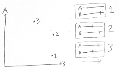
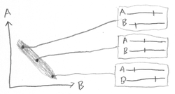
Then we can view the state of the complete system A+B as a single point in 2-dimensional space.
If you look at state 1, for example, it describes a state of the system where B is far forward and A is far back. We can view state 1 as being embodied either in two 1-dimensional positions (the representation on the right), or view it as one 2-dimensional position (the representation on the left).
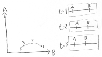
When A and B are far apart, they both move toward each other. However, B moves slower than A. Also, B wants to be closer to A than A wants to be close to B, so as B gets too close, A runs away...
(At least that’s what I had in mind while trying to draw the system evolution.)
The system evolution can be shown as a discrete series of states: Time=1, Time=2, Time=3… But in configuration space, I can draw the system evolution as a smooth trajectory.
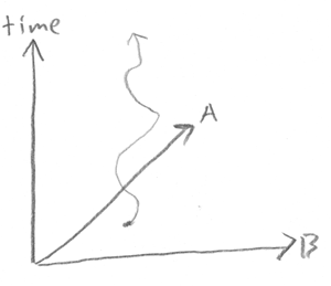
You may have previously heard the phrase, “time is the 4th dimension”. But the diagram at right shows the evolution over time of a 1-dimensional universe with two particles. So time is the third dimension, the first dimension being the position of particle A, and the second dimension being the position of particle B.
All these neat pictures are simplified, even relative to classical physics.
In classical physics, each particle has a 3-dimensional position and a 3-dimensional velocity. So to specify the complete state of a 7-particle system would require 42 real numbers, which you could view as one point in 42-dimensional space.
Hence the joke.
Configuration spaces get very high-dimensional, very fast. That’s why we’re sticking with 2 particles in a 1-dimensional universe. Anything more than that, I can’t draw on paper—you’ve just got to be able to visualize it in N dimensions.
So far as classical physics is concerned, it’s a matter of taste whether you would want to imagine a system state as a point in configuration space, or imagine the individual particles. Mathematically, the two systems are isomorphic—in classical physics, that is. So what’s the benefit of imagining a classical configuration space?
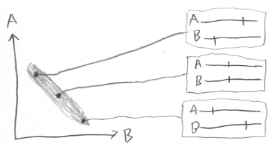
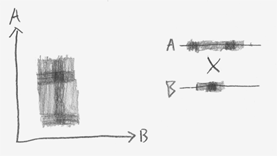
The grey area in the diagram represents a probability distribution over potential states of the A+B system.
If this is my state of knowledge, I think the system is somewhere in the region represented by the grey area. I believe that if I knew the actual states of both A and B, and visualized the A+B system as a point, the point would be inside the grey.
Three sample possibilities within the probability distribution are shown, and the corresponding systems.
And really the probability distribution should be lighter or darker, corresponding to volumes of decreased or increased probability density. It’s a probability distribution, not a possibility distribution. I didn’t make an effort to represent this in the diagram—I probably should have—but you can imagine it if you like. Or pretend that the slightly darker region in the upper left is a volume of increased probability density, rather than a fluke of penciling.
Once you’ve hit on the idea of using a bounded volume in configuration space to represent possibility, or a cloud with lighter and darker parts to represent probability, you can ask how your knowledge about a system develops over time. If you know how each system state (point in configuration space) develops dynamically into a future system state, and you draw a little cloud representing your current probability distribution, you can project that cloud into the future.
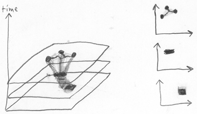
All the points in the first grey box, correspond to system states, that dynamically develop over time, into new system states, corresponding to points in the grey rectangle in the second configuration space at middle right.
Then, my little rectangle of uncertainty develops over time into a wiggly figure, three major possibility-nodes connected by thin strings of probability density, as shown at top right.
In this figure I also tried to represent the idea of conserved probability volume—the same total volume of possibility, with points evolving to other points with the same local density, at each successive time. This is Liouville’s Theorem, which is the key to the Second Law of Thermodynamics, as I have previously described.
Neat little compact volumes of uncertainty develop over time, under the laws of physics, into big wiggly volumes of uncertainty. If you want to describe the new volumes of uncertainty compactly, in less than a gazillion gigabytes, you’ve got to draw larger boundaries around them. Once you draw the new larger boundary, your uncertainty never shrinks, because probability flow is conservative. So entropy always increases. That’s the second law of thermodynamics.
Just figured I’d mention that, as long as I was drawing diagrams… you can see why this “visualize a configuration space” trick is useful, even in classical physics.
Conditional independence happens when the joint probability distribution is the product of the individual probability distributions:
P(A,B) = P(A) x P(B)
The vast majority of possible probability distributions are not conditionally independent, the same way that the vast majority of shapes are not rectangular. Actually, this is oversimplifying: It’s not enough for the volume of possibilities to be rectangular. The probability density has to factorize into a product of probability densities on each side.
The vast majority of shapes are not rectangles, the vast majority of color patterns are not plaid. It’s conditional independence, not conditional dependence, that is the unusual special case.
(I bet when you woke up this morning, you didn’t think that today you would be visualizing plaid patterns in N dimensions.)
Hence, my uncertainty about A and my uncertainty about B are not independent.
If you tell me A is far forward, I will conclude B is far back. If you tell me A is in the middle of its 1-dimensional universe, I will conclude that B is likewise in the middle.
If I tell you A is far back, what do you conclude about B?
Aaaand that’s classical configuration space, folks. It doesn’t add anything mathematically to classical physics, but it can help human beings visualize system dynamics and probability densities. It seemed worth filtering into a separate post, because configuration space is a modular concept, useful for other ideas.
Quantum physics inherently takes place in a configuration space. You can’t take it out. Tomorrow, we’ll see why.
Part of The Quantum Physics Sequence
Next post: “The Quantum Arena”
Previous post: “Can You Prove Two Particles Are Identical?”
- The Quantum Physics Sequence by (11 Jun 2008 3:42 UTC; 77 points)
- Can You Prove Two Particles Are Identical? by (14 Apr 2008 7:06 UTC; 67 points)
- Timeless Physics by (27 May 2008 9:09 UTC; 57 points)
- Decoherence by (22 Apr 2008 6:41 UTC; 43 points)
- The Quantum Arena by (15 Apr 2008 19:00 UTC; 40 points)
- And the Winner is… Many-Worlds! by (12 Jun 2008 6:05 UTC; 30 points)
- Relative Configuration Space by (26 May 2008 9:25 UTC; 22 points)
- Quantum Mechanics and Personal Identity by (12 Jun 2008 7:13 UTC; 21 points)
- Decoherence is Pointless by (29 Apr 2008 6:38 UTC; 18 points)
- An Intuitive Explanation of Quantum Mechanics by (12 Jun 2008 3:45 UTC; 18 points)
- Quantum Physics Revealed As Non-Mysterious by (12 Jun 2008 5:20 UTC; 14 points)
- [SEQ RERUN] Classical Configuration Spaces by (4 Apr 2012 4:32 UTC; 7 points)
- 's comment on Open Thread, April 1-15, 2013 by (6 Apr 2013 21:18 UTC; 2 points)
- 's comment on Living in Many Worlds by (1 Mar 2012 0:50 UTC; 0 points)
- 's comment on Designing Rationalist Projects by (15 May 2011 17:06 UTC; -59 points)
I bet when you woke up this morning, you didn’t think that today you would be visualizing plaid patterns in N dimensions.
How little you know me.
My understanding is that classical configuration space as you mentioned is usually thought of as including dimensions for velocities, or even better, momenta, in addition to positions. For even two particles in a one dimensional space, that is already four dimensions and you can’t graph it, so I can understand why you showed it the way you did. However you can show one particle, perhaps in a force field, which can be useful.
The advantage of including momentum is that a single point in configuration space has all the information needed to calculate its evolution forward (or backward) in time. A single point determines an entire trajectory (a line, or curve) in configuration space. That means that two nearby points determine two different trajectories, and in fact all of configuration space can be divided into non-intersecting trajectory lines. Only in this formulation is the Liouville Theorem true, about conservation of configuration space volumes. If you start with a certain volume in configuration space, and evolve it forward (or again, backward) in time, the volume doesn’t change. However, in most classical configurations, physics tends to be chaotic and the shape does change as you describe, developing “fingers” and “folds” and becoming very complex in structure, which leads on a crude scale to an apparent increase in the volume.
This is exactly right except that the space in which Liouville’s theorem holds is called phase space. Phase space is the cotangent bundle over configuration space; i.e., if the configuration space is an n-dimensional manifold M, then for every point in M there is a copy of an n-dimensional vector space. These n-vectors* represent momenta, and both a configuration and a momentum are necessary to uniquely specify a state of a classical (Hamiltonian) system.
* More precisely, they are one-forms—linear functions of n-vectors; i.e. they eat n-vectors and spit out scalars. One-forms are also called covariant vectors, whence the other kind are called contravariant. They are dual to each other (for a given n), and thus (contravariant) vectors can equivalently be considered linear functions of one-forms instead.
I think it would be nice if the post were edited to reflect this distinction. It wouldn’t take much effort; just a sentence inserted at the point where it switches from talking about configuration space to talking about phase space, and appropriate tweaks to a few subsequent sentences. The Wikipedia article Configuration space links here, by the way.
To clarify (seven years later), “configuration space” is the name physicists use for the space recording just the particle’s positions, and “phase space” is the name for the space recording their positions and momentums.
“I bet when you woke up this morning, you didn’t think that today you would be visualizing plaid patterns in N dimensions.”
Hrm.… When projected into 3 dimensions though, it must become the Langford mind erasing Plaid Room:
http://web.archive.org/web/20010408224421/www.lileks.com/institute/interiors/bhg/chpt8/6.html
(Be warned… once seen, it cannot be unseen. :))
If it helps, I redrew some of the diagrams (using Preview, Grapher, and the GIMP): “So time is the third dimension [...]” “[...] probability distribution over potential states of the A+B system” “[...] conditional independence between two probabilistic variables”
My father, a professor of electrical engineering, laments his students’ apparent inability to include a simple hand drawing in lab reports, instead preferring to spend hours making something using a computer.
+1 for hand drawings.
Conditional independence does not require a rectangular “cloud of uncertainty”. If you have independent normal distributions for A and B, the joint distribution—your “cloud of uncertainty”—is an axis-parallel ellipse.
At atbout n=5, I stop trying to visualize; my visual cortex just isn’t built to handle multi-dimensional spaces directly. I switch to number/symbol crunching, possibly by writing a computer program.
I looked your explanation of configuration space up when I was having trouble understanding it in the No-Nonsense Classical Mechanics book recently authored by Jakob Schwichtenberg. His book is basically a good book that mostly does what its title implies , but I thought his explanation of configuration space was very abstract and hard to understand. You cleared it up for me. Your explanation of Configuration Space is the no-nonsense explanation of CS, not his. Thanks for your work. Regards
PS: I enjoy your homemade diagrams! My opinion is don’t waste your time learning a CAD package even if people complain. If the don’t like it, rather than complain, they should volunteer to draw them for you.