Sparsify: A mechanistic interpretability research agenda
Over the last couple of years, mechanistic interpretability has seen substantial progress. Part of this progress has been enabled by the identification of superposition as a key barrier to understanding neural networks (Elhage et al., 2022) and the identification of sparse autoencoders as a solution to superposition (Sharkey et al., 2022; Cunningham et al., 2023; Bricken et al., 2023).
From our current vantage point, I think there’s a relatively clear roadmap toward a world where mechanistic interpretability is useful for safety. This post outlines my views on what progress in mechanistic interpretability looks like and what I think is achievable by the field in the next 2+ years. It represents a rough outline of what I plan to work on in the near future.
My thinking and work is, of course, very heavily inspired by the work of Chris Olah, other Anthropic researchers, and other early mechanistic interpretability researchers. In addition to sharing some personal takes, this article brings together—in one place—various goals and ideas that are already floating around the community. It proposes a concrete potential path for how we might get from where we are today in mechanistic interpretability to a world where we can meaningfully use it to improve AI safety.
Key frameworks for understanding the agenda
Framework 1: The three steps of mechanistic interpretability
I think of mechanistic interpretability in terms of three steps:
The three steps of mechanistic interpretability[1]:
Mathematical description: In the first step, we break the neural network into constituent parts, where the parts are simply unlabelled mathematical objects. These may be e.g. neurons, polytopes, circuits, feature directions (identified using SVD/NMF/SAEs), individual parameters, singular vectors of the weight matrices, or other subcomponents of a network.
Semantic description: Next, we generate semantic interpretations of the mathematical object (e.g. through feature labeling). In other words, we try to build a conceptual model of what each component of the network does.
Validation: We need to validate our explanations to ensure they make good predictions about network behavior. For instance, we should be able to predict that ablating a feature with a purported ‘meaning’ (such as the ‘noun gender feature’) will have certain predictable effects that make sense given its purported meaning (such as the network becoming unable to assign the appropriate definitive article to nouns). If our explanations can’t be validated, then we need to identify new mathematical objects and/or find better semantic descriptions.
The field of mechanistic interpretability has repeated this three-step cycle a few times, cycling through explanations given in terms of neurons, then other objects such as SVD/NMF directions or polytopes, and most recently SAE directions.
My research over the last couple of years has focused primarily on identifying the right mathematical objects for mechanistic explanations. I expect there’s still plenty of work to do on this step in the next two years or so (more on this later). To guide intuitions about how I plan to pursue this, it’s important to understand what makes some mathematical objects better than others. For this, we have to look at the description accuracy vs. description length tradeoff.
Framework 2: The description accuracy vs. description length tradeoff
You would feel pretty dissatisfied if you asked someone for a mechanistic explanation of a neural network and they proceeded to read out of the float values of the weights. But why is this dissatisfying? Two reasons:
When describing the mechanisms of any system, be it an engine, a solar system, or a neural network, there is always a tradeoff between description accuracy and description length. The network is the most accurate mathematical description of itself, but it has a very long mathematical description length.
It isn’t even a semantic description at all. This makes things difficult to understand because we can’t easily intuit mathematical descriptions. To understand what the weights in the network ‘mean’, we need semantic descriptions[2].
Part of our job in mechanistic interpretability (and the framework used in this agenda) is to push the Pareto frontier of current mechanistic interpretability methods toward methods that give us the best tradeoff between description accuracy and description length. We’re therefore not only optimizing for accurate descriptions; we’re also optimizing for shorter descriptions. In other words, we want to find objects that admit mathematical descriptions that use as few objects as possible but that capture as much of what the network is doing as possible. Furthermore, we want short semantic descriptions for these objects, such that we need few words or concepts to describe what they do.
To summarize, we’re in fact optimizing our interpretability methods according to four constraints here:
Mathematical description accuracy—How good the approximation of the original network’s behaviour is;
Mathematical description length—How many mathematical objects the network is decomposed into;
Semantic description accuracy—How good the predictions made by the conceptual model of the network are;
Semantic description length—How many words/concepts are needed to define the conceptual model of the network.
Inadequacy according to at least one of these constraints has been the downfall of several previous interpretability approaches:
Non-mechanistic approaches, such as attribution maps (e.g. Simonyan et al., 2013) have been demonstrated often to yield misleading (low accuracy) semantic descriptions (Adebayo et al., 2018; Kindermans et al., 2017).
Using neurons as the mathematical objects to interpret (e.g. Olah et al., 2020) yields too-long mathematical descriptions and even more too-long semantic descriptions due to polysemanticity.
Using SVD/NMF/ICA directions (e.g. Schubert et al., 2021; Voss et al., 2021) instead of neurons arguably improves the mathematical description length, but the semantic description length is still too long due to polysemanticity.
Using polytopes (Balestriero and Baraniuk, 2018; Black et al., 2022) as the fundamental mathematical object yields much too long mathematical descriptions[3], even if they are in some sense ‘more accurate’ with regard to the network’s nonlinear structure than directions.
This leads us to one of the core methods in this agenda that so far appears to perform well according to our four constraints: sparse autoencoders (SAEs).
The unreasonable effectiveness of SAEs for mechanistic interpretability
SAEs have risen in popularity over the last year as a candidate solution to the problem of superposition in mechanistic interpretability (Elhage et al., 2022; Sharkey et al., 2022; Cunningham et al., 2023; Bricken et al., 2023)
SAEs are very simple. They consist of an encoder (which is just a linear transformation followed by a nonlinear activation function) and a decoder (or ‘dictionary’) whose features are constrained to have fixed length. The loss function used to train them has two components: (1) The reconstruction loss, so that their output approximates their input; (2) The sparsity loss, which penalizes the encoder outputs to be sparse.
I harp on about SAEs so much that it’s become a point of personal embarrassment. But the reason is because SAEs capture so much of what we want in a mechanistic interpretability method:
The reconstruction loss trains the SAE features to approximate what the network does, thus optimizing for mathematical description accuracy.
The sparsity penalty trains the SAE to activate fewer features for any given datapoint, thus optimizing for shorter mathematical description length.
The features identified by SAEs appear more monosemantic than other methods identified so far (Cunningham et al., 2023; Bricken et al., 2023). And unlike clustering, they factorize the network’s activations into compositional components, which means they yield modular descriptions. For both these reasons, they therefore perform well according to semantic description length.
It would be nice to have a formal justification for why we should expect sparsification to yield short semantic descriptions. Currently, the justification is simply that it appears to work and a vague assumption about the data distribution containing sparse features. I would support work that critically examines this assumption (though I don’t currently intend to work on it directly), since it may yield a better criterion to optimize than simply ‘sparsity’ or may yield even better interpretability methods than SAEs.
The last selling point of SAEs that I’ll mention is that the SAE architecture and training method are very flexible: They lend themselves to variants that can be used for much more than merely identifying features in activations. For instance, they could be used to identify interactions between features in adjacent layers (sparse transcoders) or could potentially be used to identify whole circuits (meta-SAEs). We’ll have more to say about transcoders and meta-SAEs later.
Framework 3: Big data-driven science vs. Hypothesis-driven science
The last framework driving this agenda is a piece of ‘science ideology’.
In the last few decades, some branches of science have radically changed. They’ve moved away from purely hypothesis-driven science toward a ‘big data’-driven paradigm.
In hypothesis-driven science, you make an hypothesis about some phenomenon, then collect data that tests the hypothesis (e.g. through experiments or surveys). Think ‘testing general relativity’; ‘testing whether ocean temperature affects atmospheric sulfur levels’; or ‘testing whether smoking causes lung cancer’, etc.
Big Data-driven science does things differently. If Big Data-driven science had a motto, it’d be “Collect data first, ask questions later”. Big Data-driven science collects large datasets, then computationally models the structure in this data. The structure of those computational models suggests hypotheses that can be tested in the traditional way. The Big Data-driven approach has thrived in domains of science where the objects of study are too big, complex, or messy for humans to have much of a chance of comprehending it intuitively, such as genetics, computational neuroscience, or proteomics.
In mechanistic interpretability, I view work such as “Interpretability in the Wild: A Circuit for Indirect Object Identification in GPT-2 small” (Wang et al., 2023) as emblematic of ‘hypothesis-driven science’. They identified a task (‘indirect object identification’ - IOI) and asked if they could identify circuits of nodes (attention heads at particular token positions) that performed this task on a dataset they constructed. This was a very solid contribution to the field. However, to my personal research taste it felt like the wrong way to approach mechanistic interpretability in a few ways:
Is IOI a ‘task’ from the network’s perspective? Does it chop up tasks in the same way?
Are the objects studied here (attention heads at particular token indices) fundamental objects from the network’s perspective? Are any objects missing?
If we studied a different artificial dataset for a different task, would we come to different conclusions about which heads do what?
To me, it felt like coming at mechanistic interpretability from a human perspective when, instead, we should be coming at it from the network’s perspective:
We should identify tasks the way a network breaks up taskspace instead of choosing individual tasks ourselves;
Rather than choosing parts of the distribution that we think might explain the most about an hypothesis we’re currently evaluating, we should look at behavior of network components over the whole distribution and ‘let the network decide’ which are the relevant sub-distributions;
We should make hypotheses in terms of objects that the network considers fundamental, rather than deciding for ourselves what the fundamental objects are.
I contend that mechanistic interpretability is a domain that needs a Big Data-driven approach more than usual. Neural networks are too big, too messy, too unintuitive to comprehend unless we map out their components in a principled way. Without mapping the space first, we are flying blind and are bound to get lost. To be absolutely clear, Big Data-driven science does not replace hypothesis-driven science; it just augments hypothesis formation and testing. But I think that without this augmentation, mechanistic interpretability is doomed to flounder (see also Wentworth on this theme).
Fortunately, neural networks are very well suited to Big Data-driven science, because it is so easy to collect data from them. It’s even easy to directly collect data about their causal structure (i.e. information about their gradients and architecture), unlike in most areas of science!
The power of Big Data-driven science is a background assumption for much of my research. For me, it motivated the search for SAEs as a scalable, unsupervised structure-finding method, which can be applied to whole networks and datasets, and which might help reveal the objects that the network considers fundamental. It privileges big datasets that contain all the things that a network does such that, when we analyze these big datasets, the interpretable structure of the network naturally falls out thanks to unsupervised methods. And this bit of science ideology also motivates most of the objectives in the agenda.
Sparsify: The Agenda
I envision a mechanistic interpretability tech tree something like this:
I’ll explain what each of the objectives here mean in more detail below. The main convergent objective of the agenda is satisfactory whole-network mechanistic interpretability, which I think could open up a range of safety-relevant applications. Most of the other objectives can be framed as trying to improve our mathematical and semantic descriptions by improving their accuracy vs. length Pareto frontiers.
The objectives for my research over the next 2+ years are the following (with high-variance estimates for timelines that feel somewhat achievable for a community of researchers):
Objective 1: Improved SAEs: Get good at taking features out of superposition using SAEs by pushing the Pareto frontier of our mathematical descriptions closer to optimal and reducing computational costs. (Starting in 0 Months—until 1y)
Objective 2: Decompiled networks: Networks that do computation in the feature basis. (Starting in 2 months—until 1.5y)
Objective 3: Abstraction above raw decompilations: Identify circuits and, if necessary for short enough descriptions, make principled abstractions above the mechanistic layer of abstraction. (Starting in 3 months—until 2y)
Objective 4: Deep Description: Going beyond automated feature labeling by integrating different kinds of description together. (Starting in 6 months—until future)
Objective 5: Applications of mechanistic interpretability: Including mechanistic interpretability-based evals; alignment method profiling; capability prediction; and, potentially, robust to training mechanistic interpretability. (Starting 6 months—until future)
Objective 1: Improving SAEs
I think there’s lots of room for improvement on current SAEs. In particular,
Benchmarking SAEs
Fixing SAE pathologies
Applying SAEs to attention
Better hyperparameter selection methods
Computationally efficient sparse coding
Benchmarking SAEs
At present, it’s difficult to know when SAEs should be considered ‘good’. We need to devise principled metrics and standardized ways to compare them. This will be important both for identifying good SAEs trained on models and for developing improvements on SAEs and SAE training methods.
Fixing SAE pathologies
Current SAEs exhibit a few pathologies that make them suboptimal as mathematical descriptions in terms of both description accuracy and description length. My collaborators and I (through MATS and Apollo Research) are working on a few posts that aim to address them. Here we share an overview of a few early results:
Finding functionally relevant features using e2e SAEs (link) (Dan Braun, Jordan Taylor, Nix Goldowsky-Dill, Lee Sharkey): There is no guarantee that the directions that SAEs find are ‘functionally relevant’ to the network; SAEs currently just find directions that reconstruct a layer’s activations well while being sparse. We demonstrate that the standard reconstruction loss used to train SAEs is not optimal for learning functionally relevant features and show that an end-to-end (e2e) loss function, which reconstructs activations and distributions in later layers, improves the functional relevance of the features learned. End-to-end training means a smaller, more accurate set of SAE features can explain the same amount of network function, implying the typical way of training SAEs is suboptimal according to mathematical description accuracy and length.
Choosing better sparsity penalties than L1 (Upcoming post - Ben Wright & Lee Sharkey): There is reason to believe that is a suboptimal sparsity penalty: In toy datasets, where we know the ground truth features, an penalty leads to too many features being learned compared with ground truth features. This leads to suboptimal mathematical description length. We propose a simple fix: Use instead of , which seems to be a Pareto improvement over (at least in some real models, though results might be mixed) in terms of the number of features required to achieve a given reconstruction error.
Addressing feature suppression (link)(Ben Wright & Lee Sharkey): When SAE encoders guess how much of a feature is present in their input, they systematically undershoot. This is due to their optimizing both reconstruction and , resulting in suboptimal mathematical description accuracy. Ben looked at a way to fix this undershooting. We think success, while real, was modest. We think there are probably ways to improve upon the results of this work.
Applying SAEs to attention
Some work (unrelated to my collaborators and I) demonstrate that SAEs work reasonably well when applied to attention block outputs (Kissane et al., 2024). However, so far, the inner workings of attention blocks remain somewhat enigmatic and attention head superposition (Jermyn et al., 2023) remains unresolved.
How best to apply SAE-like methods to decompose attention blocks? We have investigated two approaches in parallel:
Gated Attention Blocks: Preliminary Progress toward Removing Attention Head Superposition (link) (Chris Mathwin, Dennis Akar, Lee Sharkey). Here, Chris Mathwin studies a particular kind of attention head superposition that involves constructive and destructive interference between the outputs of different attention heads, studied by Jermyn et al. (2023). The post introduces a gated attention block, which is a type of transcoder (see Objective 2 below for further explanation) for attention blocks, that resolves this kind of attention head superposition in a toy model.
Decomposing attention block jobs and identifying QK-circuit features with sparse transcoders (link)(Keith Wynroe and Lee Sharkey): Keith Wynroe has been taking a different approach, using transcoders that are more similar to vanilla SAEs than Chris’ gated attention blocks. In Keith’s work, the features learned are in the QK circuit, and they are not trained on reconstruction of activations, but are instead trained to reconstruct the attention pattern. We use these features to construct a third-order tensor whose structure (we hope) reflects the various QK-‘jobs’ done by the attention block. Another type of sparse factorization is used on this ‘attention head jobs tensor’ to break it into (what we hope will be) individual attention block ‘jobs’.
Better hyperparameter selection methods
Training SAEs requires selecting multiple hyperparameters. We don’t know how hyperparameters interact with each other, or how they interact with different data distributions. Thus training SAEs often involves sweeps over hyperparameters to find good combinations. Understanding the relationships between different hyperparameters (similar to Yang et al., (2022)) would let us skip expensive hyperparameter sweeps. This is especially important as we scale our interpretability methods to frontier models, where it may be prohibitively expensive to run SAE hyperparameter sweeps.
Computationally efficient sparse coding
There may be additional tips and tricks for training SAEs in more efficient ways. For instance, informed initialization schemes (such as data initialization or resampling) may improve efficiency. Or perhaps particular methods of data preprocessing might help. There is considerable room for exploration.
On a higher level, there probably exist more efficient sparse coding methods than SAEs trained with SGD. If there are better methods, it’s important that the community not get stuck in a local optimum; we should look for these better methods.
In order to be in a position where the next objective is completable, we would need to see some progress in the above areas. Areas of progress like ‘better hyperparameter selection’ and ‘computational efficiency’ would yield quality of life improvements. Others are more important; they are essential before we can be confident in our descriptions: Areas like ‘finding functionally relevant features’ or ‘fixing feature suppression’. Other still are even more essential for progress: Unless we can decompose attention blocks in a satisfying way, we will not be able to complete the next objective, which is to fully ‘decompile networks’.
Objective 2: Decompiled networks
Once we’ve identified the functional units of a neural network, then we can decompile it by making a version of the network where superposition has been removed. In decompiled networks, the forward pass does inference in the interpretable feature basis.
Suppose we have trained e2eSAEs in each layer and identified the functional units. We then want to identify the ‘interaction graph’ that describes how features interact between layers. This is where ‘transcoders’ come in. Transcoders, in contrast to autoencoders, are trained to produce different outputs than their inputs. To get the interaction graph between features in adjacent layers, we would train (or otherwise find, perhaps through cleverly transforming the original network’s parameters into sparse feature space) a set of transcoders to produce the same output and intermediate feature activations as in the original network. The result is a sparse model that we can use for inference where we don’t need to transform our activations to the original neuron basis; the decompiled network does inference entirely in the sparse feature basis.
Transcoders may have a variety of architectures, such as a simple matrix (as in Riggs et al., 2024 and Marks et al., 2024). Speculatively, we may prefer using something else, such as another SAE architecture (as briefly explored in Riggs et al., 2024). Unlike a purely linear transcoder, an SAE-architecture-transcoder would be able to model nonlinear feature interactions.
It’s worth noting that such a transcoder’s sparsely activating features would be ‘interaction features’, which identify particular combinations of sparse features in one layer that activate particular combinations of sparse features in the next layer. The weights of these interaction features are the ‘interaction strengths’ between features. You can thus study the causal influence between features in adjacent layers by inspecting the weights of the transcoder, without even needing to perform causal intervention experiments. The transcoder’s interaction features thus define the ‘atomic units’ of counterfactual explanations for the conditions under which particular features in one layer would activate features in an adjacent layer.
Policy goals for network decompilation
Once we as a community get network decompilation working, we hope that it becomes a standard for developers of big models to produce decompiled versions of their networks alongside the original, ‘compiled’ networks. Some of the arguments for such a standard are as follows:
Certain highly capable models will be integrated widely into society and used for economically gainful activities. This comes with some risks, which would be reduced by the existence of decompiled models that are easier to understand.
Developers of large models are best placed to train the decompiled versions themselves, since they have access to the training resources and infrastructure.
This standard would mean that, as neural networks scale, auditors and researchers would always have a version of the network that is ready for interpretation.
It is not unreasonable for developers to internalize some of the costs associated with big models by training interpretable decompiled versions of them in addition to the base models, so that researchers can work on ensuring that the original model is safe.
Standardized artifacts enable standardized tests: Evaluators could, for example, run standardized tests for particular knowledge in the network, or test for signatures of dangerous cognitive capabilities, or test for particular biases.
Standardized artifacts enable cumulative policy development. For instance, regulators could begin designing regulations that require the networks to have particular internal properties, as identified in their decompiled networks. We might even be able to graduate from risk-management-based AI safety assurances to compliance-based AI safety assurances.
Objective 3: Abstraction above raw decompilations
Although we expect decompiled neural networks to be much more interpretable than the original networks, we may wish to engage in further abstractions for two reasons:
Circuit identification: We may wish to identify ‘circuits’, i.e. modules within a neural network that span multiple layers consisting of groups of causally interacting features that activate together to serve a particular function. If we identify circuits in a principled way, then they represent a natural way to study groups of features and interactions in the network.
Shorter semantic descriptions: If semantic descriptions of neural networks in terms of the lowest level features are too long, then we need to identify the right abstractions for our lowest-level objects and then describe networks one level of abstraction up.
The best abstractions are those that reduce [mathematical or semantic] description length as much as possible while sacrificing as little [mathematical or semantic] description accuracy as possible. We previously used sparse coding for this exact purpose (see section The Unreasonable Effectiveness of SAEs for Mechanistic interpretability), so perhaps we can use them for that purpose again. So, at risk of losing all personal credibility to suggest it, SAEs may be reusable on this level of abstraction[4]. It may be possible to train meta-SAEs to identify groups of transcoder features (which represent interactions between SAE features) that commonly activate together in different layers of the network (figure 5). The transcoder features in different layers could be concatenated together to achieve this, echoing the approach taken by Yun et al. (2021) (although they did not apply sparse coding to interactions between features in decompiled networks, only to raw activations at each layer). Going further still, it may be possible to climb to higher levels of abstraction using further sparse coding, which might describe interactions between circuits, and so on.
Objective 4: Deep Description
So far in this agenda, we haven’t really done any (semantic) ‘interpretation’ of networks. We’ve simply decompiled the networks, putting them in a format that’s easier to interpret. Now we’re ready to start semantically describing what the different parts of the decompiled network actually do.
In mechanistic interpretability, we want a mechanistic description of all the network’s features and their interactions. On a high level, it’s important to ask what we’re actually looking for here. What is a mechanistic description of a feature?
A complete mechanistic description of a feature is ideally a description of what causes it to activate and what it subsequently does. Sometimes it makes sense to describe what a feature does in terms of which kinds of input data make it activate (e.g. feature visualization, Olah et al., 2017). Other times it makes more sense to describe what a feature does in terms of the output it tends to lead to. Other times still, it is hard or incomplete to describe things in terms of either the input or output, and instead it only makes sense to describe what a feature does in terms of other hidden features.
There exists some previous work that aims to automate the labeling of features (e.g. Bills et al., 2023). But this work has only described neurons in terms of either the input or output of the network. These descriptions are shallow. Instead, we want deep descriptions. Deep descriptions iteratively build on shallow descriptions and bring in information about how features connect together and participate in particular circuits together.
Early ventures into deep description have already been made, but there is potentially much, much further to go. One of these early ventures is Cammarata et al. (2021) (Curve Circuits). In this work, they used feature visualization to get a first pass of shallow descriptions of all the relevant neurons. In the next iteration of description, they showed how features in one layer get used by particular weights to construct features in the next layer; in doing so, they showed that some ‘curve features’ were not merely excited by curves in particular orientations, but also inhibited by curves in opposite orientations, thus adding more semantic detail.
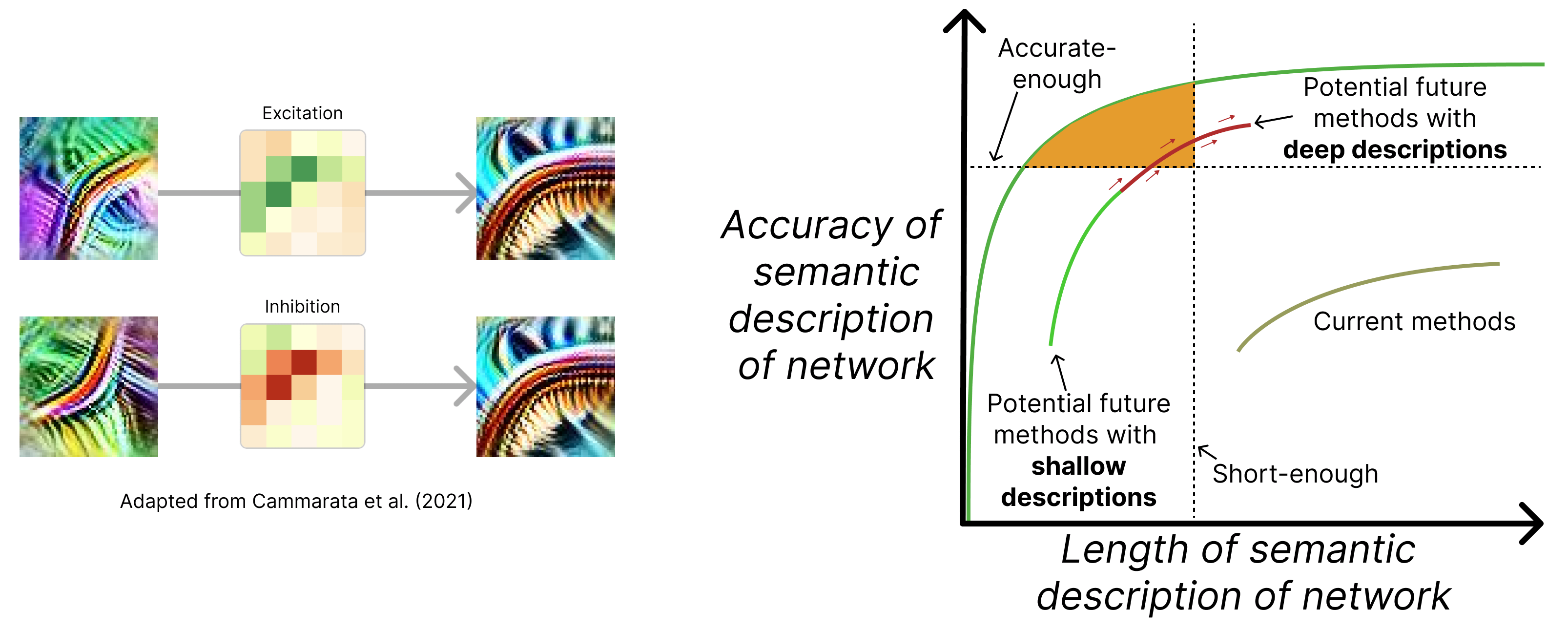
This foray into deep description showed how we can use descriptions to build on each other iteratively. But these were only an initial step into deep description. This example only explained a hidden feature (a curve) in terms of features (early curves) in a previous layer; it didn’t, for instance, ‘go backward’, explaining early curves in terms of the curves they participate in. Being so early in the network, this might not be as informative an exercise as going in the forward direction. But there will exist features, particularly those toward the output of the network, where it makes more sense to go in the backwards direction, explaining hidden features in terms of their downstream causes.
What description depths might we be able to achieve if we automate the description process, and what might automating such a process look like? Here is a sketch for how we might automate deeper description.
A sketch of an automated process for deep description: The Iterative-Forward-Backwards procedure
This procedure has three loops. Intuitively:
The ‘Forward loop’ describes features in one layer in terms of features in earlier layers or in terms of the data. It describes what causes feature X to fire in terms of earlier features.
The ‘Backward loop’ describes features in one layer in terms of features in later layers or in terms of the output. It describes the effects in later layers caused by feature X activating.
The ‘Iterative loop’ lets us use the results of previous cycles to iteratively refine our descriptions based on descriptions that have previously been added, developed, or clarified.
Suppose we have a network with L layers (where layer 0 is the input data and L is the output layer) and a number of repeats for the iterative loop, R. Then, slightly more formally:
For r in (0, …, R-1):  #  The Iterative loop
	For i in(0, …, L):  #  The Forward loop
		For j in (1, …, L):
			If i < j:
				Explain the features in layer j in terms of the (earlier) features in layer i.
	For k in (L, …, 1):  #  The Backward loop
		For j’ in (L, …, 0):
			If k > j’:
				Explain the features in layer j’ in terms of the (later) features in layer k.
When we say ‘Explain feature X in terms of features Y’, we’re leaving a lot undefined. This step is doing a lot of work. It may take several forms. For instance:
It potentially involves looking at the max activating samples of feature X. If Y is the data, then we’d look at the data and which data caused X to activate a lot. But note that Y may be hidden features too.
It could involve testing hypotheses about our descriptions of features X in terms of Y. For example, we could look at the features X and the weights that connect features Y to them and make predictions about the activations of features Y that would cause features X to activate as in Bills et al. (2023).
It could involve predicting the outcomes of particular causal interventions on features, as in causal scrubbing.
To add to the intuitions of what this procedure is doing, it is helpful to describe previous interpretability methods in terms of it (Figure 6):
Feature visualization-based methods (e.g. activation atlases or max-activating dataset-examples) are instances of one part of the forward loop, where layer l is explained in terms of layer 0 (the input layer).
The logit lens is an instance of one part of the backwards loop, where features in hidden layer j’ are explained in terms of the output it corresponds to.
The low level explanations of curve circuits in Cammarata et al. (2021) are instances of one step of the forward loop, where hidden layer features are explained in terms of earlier hidden layer features. This occurs during the first iterative loop, since the explanations for each feature are simply given only in terms of layer 0 (the input data). Subsequent iterative loops would be able to make use of much more information.
I expect the procedure that we end up doing to look substantially different from this (and include a lot more detail). But this sketch is merely supposed to point toward algorithms that could let us automate a lot of semantic description in interpretability.
Objective 5: Mechanistic interpretability-based evals & other applications of mechanistic interpretability
If we figure out how to automate deep description of decompiled networks, then we’ll have satisfactory mechanistic interpretability. This could be used for a number of applications, including:
Mechanistic interpretability-based model evaluations: We can develop red-teaming procedures and benchmarks based on our mechanistic interpretability methods to assess the safety and ethics of the models’ internal representations and learned algorithms. These would be a type of ‘understanding-based model evals’. Not only could these evals permit new kinds of model capability evals, they may also permit more general alignment evals, where we can make good predictions of how models would behave on a much wider range of circumstances than current behavioral model evals.
We think of mech-interp based model evaluations as falling into two broad categories:Mechanistic interpretability-based model red teaming: Red-teaming AI models involves trying to find inputs that fail some safety- or security-based test. Currently, most red-teaming involves searching through input-space (or latent space) to find inputs (or potential inputs) that lead to concerning outputs (e.g. Perez et al., 2022). Mechinterp-based evals can aim to do better in a couple of ways:
1) Mechanistic interpretability-based evals could try to find inputs that lead to concerning combinations of features. For example, we could try to find inputs that elicit deception that we wouldn’t have been able to detect using behavioral tests alone;
2) Mechanistic interpretability-based evals don’t have to look for inputs that cause concerning hidden feature activations or outputs (which may be difficult to enumerate for large networks). We can find (earlier) hidden features that activate concerning (later) hidden features or outputs. We could subsequently use these earlier hidden features to find even earlier hidden features that cause concerning behavior. This might even let us work backwards from hidden features, potentially using this approach as a tool to find inputs that lead to concerning behavior.
Mechanistic interpretability-based model benchmarking: Behavioral benchmarks are standardized sets of tests where, given a certain input, the output of a model is evaluated. If it’s the ‘right’ kind of output (according to some evaluation criteria), then the model does well on the benchmark. In mechanistic interpretability-based benchmarks, instead of assessing outputs, we assess internal activations. We’d similarly use some evaluation criteria to determine whether the input caused the ‘right’ kind of internal activations to occur.
Alignment method evaluations: When we have mechanistic interpretability-based model evaluations to assess model’s safety properties, we would then be able to better compare the strengths and weaknesses of different alignment methods. We may be able to strengthen different approaches by using mechinterp-based model evals to, e.g. identify key gaps in the finetuning data that lead to failures of alignment.
Targeted interventions on models: When we understand how models work, it seems likely that we can use this information to make targeted interventions on models. For instance, we may be able to:
Accurately ablate specific pieces of knowledge (e.g. for anonymization purposes or for removing unsafe capabilities);
Whitelist only a small set of capabilities, giving us better guarantees about how models will behave on specific distributions;
Make better probes that use features (i.e. causal components of the network’s internal mechanisms) rather than probes identified using correlations on a training dataset; or
Identify better steering vectors for activation steering, thus affording us more control over model behavior.
Capability prediction: One of the problems with behavioral evals is that just because we can’t get a model to behave badly or exhibit a certain capability, doesn’t mean there don’t exist ways to get it to do so; we just haven’t found them yet. In other words, ‘Absence of evidence is not evidence of absence’. Mechinterp-based evals might alleviate this problem by providing us with a way to predict capabilities and more convincingly determine whether systems can plausibly exhibit dangerous behaviors under some circumstances. For instance, if we observe that a model has all the requisite representations for particular cyber offensive capabilities, we could predict that there might exist some contexts where the model would use those capabilities even though we haven’t yet identified a way to elicit them.
Mechanistic interpretability during training: One of the barriers to doing many mechinterp-based evals during training is that it first involves interpreting a snapshot of the model. By default, this might be too expensive to do with high frequency. Nevertheless, we’d like to be able to do interpretability during training in order to e.g. better catch misalignment or dangerous capabilities before risks are realized, or to forecast discontinuities in training. We would therefore like to do mechanistic interpretability as frequently as possible. We will need efficient mechanistic interpretability methods to do this. In the long term, a potential approach might be ‘stateful interpretability’, where e.g. our semantic descriptions of features and interactions are stored as embedding vectors (a ‘state’) and, conditioned on a gradient update of the model being trained, we use another model to incrementally update the interpretation embeddings alongside the model updates.
Robust-to-training mechanistic interpretability: Once we have sufficiently good and sufficiently cheap mechanistic interpretability, one possible use is to ‘train models against the interpretability methods’. For example, if we identify features or circuits that we don’t like, we could design loss functions (or other feedback functions) that penalize the network for having them. One risk is that our interpretability methods are not ‘robust to training’ against them (Hubinger et al., 2022), so networks might simply learn to represent the features or circuits in some other, uninterpretable way (Sharkey, 2022). It remains an open question whether future interpretability methods will be robust enough for this. This debate can probably be resolved empirically before its potential use in highly capable, potentially deceptive models.
I think AI safety would be in a pretty great place if we achieved these objectives. And, to me, most feel within reach—even on reasonably short timelines—though not for a single researcher or even a single research team. It will require a concentrated research program and an ecosystem of researchers. I hope some of them will find this roadmap useful. I plan to work on it over the next few years, although some deviations are inevitable. And if others are interested in collaborating on parts of it, I’d love to hear from you! Send me a message or join the #sparse-autoencoders channel on the Open Source Mechanistic Interpretability Slack workspace.
Acknowledgements: I’m very grateful for helpful discussions and useful feedback and comments on previous drafts, which greatly improved the quality of this post, from Marius Hobbhahn, Daniel Braun, Lucius Bushnaq, Stefan Heimersheim, Jérémy Scheurer, Jordan Taylor, Jake Mendel, and Nix Goldowsky-Dill.
- ^
The analogy between mechanistic interpretability and software reverse engineering
Mechanistic interpretability has been compared to software reverse engineering, where you start with a compiled program binary and try to reconstruct the software’s source code. The analogy is that a neural network is a program that we have to decompile and reverse engineer. On a high level, software reverse engineering comprises three steps, which (not coincidentally) neatly map onto the three steps of mechanistic interpretability:
The three steps of Software Reverse engineering
1) Information extraction: In the first step, you gather what information you can that might help you understand what the program is doing. It might involve the use of a ‘disassembler’, breaks the program into its constituent parts by converting binary code into assembly code or converting machine language into a user friendly format (source). Or it may involve gathering other information such as design documents.
2) Conceptual modeling: Using the gathered information, create a conceptual model of what the program is doing. Software reverse engineering may implement this conceptual model in code that they write themselves or as a flow diagram.
3) Review: Then the conceptual model is validated to check how well it explains the original program. If it performs well, then there’s no need to keep going. If it performs poorly, then either new information will need to be extracted and/or a new conceptual model built.
- ^
To the best of my understanding, ARC’s work on heuristic arguments could be described as aiming to formalize semantic description. This seems like a very good idea.
- ^
Previous interpretability research that aimed to use polytopes as the unit of explanation(Black et al., 2022) grouped polytopes using clustering methods, which, unlike SAEs, offer no way to ‘factorize’ a network’s function into compositional components. This yielded too long mathematical descriptions. However, it may be possible to group polytopes using other methods that are more compositional than clustering.
- ^
Although meta-SAEs might be useful here, it may not be advisable to use them. The inputs to meta-SAEs may become too wide for computational tractability, for instance. Alternatively, there may simply be better tools available: Meta-SAEs are solving a slightly different optimization problem compared with base/feature-level SAEs; on the base level, they’re solving a sparse optimization problem (where we’re looking for sparsely activating features in neural activations); on the meta-SAE level, it’s a doubly sparse optimization problem (where we’re looking for sparsely activating combinations of sparse feature activations). It’s plausible that other unsupervised methods are better suited to this task.
- Shallow review of technical AI safety, 2024 by (29 Dec 2024 12:01 UTC; 202 points)
- You can remove GPT2’s LayerNorm by fine-tuning for an hour by (8 Aug 2024 18:33 UTC; 166 points)
- Apollo Research 1-year update by (29 May 2024 17:44 UTC; 93 points)
- Dmitry’s Koan by (10 Jan 2025 4:27 UTC; 44 points)
- (Maybe) A Bag of Heuristics is All There Is & A Bag of Heuristics is All You Need by (3 Oct 2024 19:11 UTC; 41 points)
- Mech Interp Lacks Good Paradigms by (16 Jul 2024 15:47 UTC; 40 points)
- Compositionality and Ambiguity: Latent Co-occurrence and Interpretable Subspaces by (20 Dec 2024 15:16 UTC; 36 points)
- Standard SAEs Might Be Incoherent: A Choosing Problem & A “Concise” Solution by (30 Oct 2024 22:50 UTC; 27 points)
- Bridging the VLM and mech interp communities for multimodal interpretability by (28 Oct 2024 14:41 UTC; 19 points)
- 's comment on StefanHex’s Shortform by (20 Nov 2024 20:15 UTC; 9 points)
- 's comment on Transcoders enable fine-grained interpretable circuit analysis for language models by (2 May 2024 18:45 UTC; 2 points)
It makes me a bit worried that this post seems to implicitly assume that SAEs work well at their stated purpose. This seems pretty unclear based on the empirical evidence and I would bet against.[1]
It also seems to assume that “superposition” and “polysemanticity” are good abstractions for understanding what’s going on. This seems at least unclear to me, though it’s probably at least partially true.
(Precisely, I would bet against “mild tweaks on SAEs will allow for interpretability researchers to produce succinct and human understandable explanations that allow for recovering >75% of the training compute of model components”. Some operationalizations of these terms are explained here. I think people have weaker hopes for SAEs than this, but they’re trickier to bet on.)
If I was working on this research agenda, I would be very interested in either:
Finding a downstream task that demonstrates that the core building block works sufficiently. It’s unclear what this would be given the overall level of ambitiousness. The closest work thus far is this I think.
Demonstrating strong performance at good notions of “internal validity” like “we can explain >75% of the training compute of this tiny sub part of a realistic LLM after putting in huge amounts of labor” (>75% of training compute means that if you scaled up this methodology to the whole model you would get performance which is what you would get with >75% of the training compute used on the original model). Note that this doesn’t correspond to reconstruction loss and instead corresponds to the performance of human interpretable (e.g. natural language) explanations.
To be clear, the seem like a reasonable direction to explore and they very likely improve on the state of the art in at least some cases. It’s just that they don’t clearly work that well at an absolute level.
Thanks for this feedback! I agree that the task & demo you suggested should be of interest to those working on the agenda.
There were a few purposes proposed, and at multiple levels of abstraction, e.g.
The purpose of being the main building block of a mathematical description used in an ambitious mech interp solution
The purpose of being the main building block of decompiled networks
The purpose of taking features out of superposition
I’m going to assume you meant the first one (and maybe the second). Lmk if not.
Fwiw I’m not totally convinced that SAEs are the ultimate solution for the purposes in the first two bullet points. But I do think they’re currently SOTA for ambitious mech interp purposes, and there is usually scientific benefit of using imperfect but SOTA methods to push the frontier of what we know about network internals. Indeed, I view this as beneficial in the same way that historical applications of (e.g.) causal scrubbing for circuit discovery were beneficial, despite the imperfections of both methods.
I’ll also add a persnickety note that I do explicitly say in the agenda that we should be looking for better methods than SAEs: “It would be nice to have a formal justification for why we should expect sparsification to yield short semantic descriptions. Currently, the justification is simply that it appears to work and a vague assumption about the data distribution containing sparse features. I would support work that critically examines this assumption (though I don’t currently intend to work on it directly), since it may yield a better criterion to optimize than simply ‘sparsity’ or may yield even better interpretability methods than SAEs.”
However, to concede to your overall point, the rest of the article does kinda suggest that we can make progress in interp with SAEs. But as argued above, I’m comfortable that some people in the field proceed with inquiries that use probably imperfect methods.
I’m curious if you believe that, even if SAEs aren’t the right solution, there realistically exists a potential solution that would allow researchers to produce succinct, human understandable explanation that allow for recovering >75% of the training compute of model components?
I’m wondering if the issue you’re pointing at is the goal rather than the method.
There isn’t any clear reason to think this is impossible, but there are multiple reasons to think this is very, very hard.
I think highly ambitious bottom up interpretability (which naturally pursues this sort of goal), seems like an decent bet overall, but seems unlikely to succeed. E.g. more like a 5% chance of full ambitious success prior to the research[1] being massively speed up by AI and maybe a 10% chance of full success prior to humans being obsoleted.
(And there is some chance of less ambitious contributions as a byproduct of this work.)
I just worried because the field is massive and many people seem to think that the field is much further along than it actually is in terms of empirical results. (It’s not clear to me that we disagree that much, especially about next steps. However, I worry that this post contributes to a generally over optimistic view of bottom-up interp that is relatively common.)
The research labor, not the interpretability labor. I would count it as success if we know how to do all the interp labor once powerful AIs exist.
It seems worth noting that there are good a priori reasons to think that you can’t do much better than around the “size of network” if you want a full explanation of the network’s behavior. So, for models that are 10 terabytes in size, you should perhaps be expecting a “model manual” which is around 10 terabytes in size. (For scale this is around 10 million books as long as moby dick.)
Perhaps you can reduce this cost by a factor of 100 by taking advantage of human concepts (down to 100,000 moby dicks) and perhaps you can only implicitly represent this structure in a way that allow for lazy construction upon queries.
Or perhaps you don’t think you need something which is close in accuracy to a full explanation of the network’s behavior.
More discussion of this sort of consideration can be found here.
Yep, that seems reasonable.
I’m guessing you’re not satisfied with the retort that we should expect AIs to do the heavy lifting here?
I think the accuracy you need will depend on your use case. I don’t think of it as a globally applicable quantity for all of interp.
For instance, maybe to ‘audit for deception’ you really only need identify and detect when the deception circuits are active, which will involve explaining only 0.0001% of the network.
But maybe to make robust-to-training interpretability methods you need to understand 99.99...99%.
It seem likely to me that we can unlock more and more interpretability use cases by understanding more and more of the network.
I think this presents a plausible approach and is likely needed for ambitious bottom up interp. So this seems like a reasonable plan.
I just think that it’s worth acknowledging that “short description length” and “sparse” don’t result in something which is overall small in an absolute sense.
I’m confused by this claim and some related ones, sorry if this comment is correspondingly confused and rambly.
It’s not obvious at all to me that SAEs lead to shorter descriptions in any meaningful sense. We get sparser features (and maybe sparser interactions between features), but in exchange, we have more features and higher loss. Overall, I share Ryan’s intuition here that it seems pretty hard to do much better than the total size of the network parameters in terms of description length.
Of course, the actual minimal description length program that achieves the same loss probably looks nothing like a neural network and is much more efficient. But why would SAEs let us get much closer to that? (The reason we use neural networks instead of arbitrary Turing machines in the first place is that optimizing over the latter is intractable.)
One might say that SAEs lead to something like a shorter “description length of what happens on any individual input” (in the sense that fewer features are active). But I don’t think there’s a formalization of this claim that captures what we want. In the limit of very many SAE features, we can just have one feature active at a time, but clearly that’s not helpful.
If you’re fine with a significant hit in loss from decompiling networks, then I’m much more sympathetic to the claim that you can reduce description length. But in that case, I could also reduce the description length by training a smaller model.
You might also be using a notion of “mathematical description length” that’s a bit different from what I’m was thinking of (which is roughly “how much disk space would the parameters take?”), but I’m not sure what it is. One attempt at an alternative would be something like “length of the shortest efficiently runnable Turing machine that outputs the parameters”, in order to not penalize simple repetitive structures, but I have no idea how using that definition would actually shake out.
All that said, I’m very glad you wrote this detailed description of your plans! I’m probably more pessimistic than you about it but still think this is a great post.
Thanks Erik :) And I’m glad you raised this.
One of the things that many researchers I’ve talked to don’t appreciate is that, if we accept networks can do computation in superposition, then we also have to accept that we can’t just understand the network alone. We want to understand the network’s behaviour on a dataset, where the dataset contains potentially lots of features. And depending on the features that are active in a given datum, the network can do different computations in superposition (unlike in a linear network that can’t do superposition). The combined object ‘(network, dataset)’ is much larger than the network itself.
ExplanationsDescriptions of the (network, dataset) object can actually be compressions despite potentially being larger than the network.So,
You can have one feature active for each datapoint, but now we’ve got an
explanationdescription of the (network, dataset) that scales linearly in the size of the dataset, which sucks! Instead, if we look for regularities (opportunities for compression) in how the network treats data, then we have a better chance atexplanationsdescriptions that scale better with dataset size. Suppose a datum consists of a novel combination of previouslyexplaineddescribed circuits. Then ourexplanationdescription of the (network, dataset) is much smaller than if weexplaineddescribed every datapoint anew.In light of that, you can understand my disagreement with “in that case, I could also reduce the description length by training a smaller model.” No! Assuming the network is smaller yet as performant (therefore presumably doing more computation in superposition), then the
explanationdescription of the (network, dataset) is basically unchanged.Is there some formal-ish definition of “explanation of (network, dataset)” and “mathematical description length of an explanation” such that you think SAEs are especially short explanations? I still don’t think I have whatever intuition you’re describing, and I feel like the issue is that I don’t know how you’re measuring description length and what class of “explanations” you’re considering.
As naive examples that probably don’t work (similar to the ones from my original comment):
We could consider any Turing machine that approximately outputs (network, dataset) an “explanation”, but it seems very likely that SAEs aren’t competitive with short TMs of this form (obviously this isn’t a fair comparison)
We could consider fixed computational graphs made out of linear maps and count the number of parameters. I think your objection to this is that these don’t “explain the dataset”? (but then I’m not sure in what sense SAEs do)
We could consider arithmetic circuits that approximate the network on the dataset, and count the number of edges in the circuit to get “description length”. This might give some advantage to SAEs if you can get sparse weights in the sparse basis, seems like the best attempt out of these three. But it seems very unclear to me that SAEs are better in this sense than even the original network (let alone stuff like pruning).
Focusing instead on what an “explanation” is: would you say the network itself is an “explanation of (network, dataset)” and just has high description length? If not, then the thing I don’t understand is more about what an explanation is and why SAEs are one, rather than how you measure description length.
ETA: On re-reading, the following quote makes me think the issue is that I don’t understand what you mean by “the explanation” (is there a single objective explanation of any given network? If so, what is it?) But I’ll leave the rest in case it helps clarify where I’m confused.
I’ll register that I prefer using ‘description’ instead of ‘explanation’ in most places. The reason is that ‘explanation’ invokes a notion of understanding, which requires both a mathematical description and a semantic description. So I regret using the word explanation in the comment above (although not completely wrong to use it—but it did risk confusion). I’ll edit to replace it with ‘description’ and strikethrough ‘explanation’.
“explanation of (network, dataset)”: I’m afraid I don’t have a great formalish definition beyond just pointing at the intuitive notion. But formalizing what an explanation is seems like a high bar. If it’s helpful, a mathematical description is just a statement of what the network is in terms of particular kinds of mathematical objects.
“mathematical description length of an explanation”: (Note: Mathematical descriptions are of networks, not of explanations.) It’s just the set of objects used to describe the network. Maybe helpful to think in terms of maps between different descriptions: E.g. there is a many-to-one map between a description of a neural network in terms of polytopes and in terms of neurons. There are ~exponentially many more polytopes. Hence the mathematical description of the network in terms of individual polytopes is much larger.
I would not. So:
I think that the confusion might again be from using ‘explanation’ rather than description.
SAEs (or decompiled networks that use SAEs as the building block) are supposed to approximate the original network behaviour. So SAEs are mathematical descriptions of the network, but not of the (network, dataset). What’s a mathematical description of the (network, dataset), then? It’s just what you get when you pass the dataset through the network; this datum interacts with this weight to produce this activation, that datum interacts with this weight to produce that activation, and so on. A mathematical description of the (network, dataset) in terms of SAEs are: this datum activates dictionary features xyz (where xyz is just indices and has no semantic info), that datum activates dictionary features abc, and so on.
Lmk if that’s any clearer.
Thanks for the detailed responses! I’m happy to talk about “descriptions” throughout.
Trying to summarize my current understanding of what you’re saying:
SAEs themselves aren’t meant to be descriptions of (network, dataset). (I’d just misinterpreted your earlier comment.)
As a description of just the network, SAEs have a higher description length than a naive neuron-based description of the network.
Given a description of the network in terms of “parts,” we can get a description of (network, dataset) by listing out which “parts” are “active” on each sample. I assume we then “compress” this description somehow (e.g. grouping similar samples), since otherwise the description would always have size linear in the dataset size?
You’re then claiming that SAEs are a particularly short description of (network, dataset) in this sense (since they’re optimized for not having many parts active).
My confusion mainly comes down to defining the words in quotes above, i.e. “parts”, “active”, and “compress”. My sense is that they are playing a pretty crucial role and that there are important conceptual issues with formalizing them. (So it’s not just that we have a great intuition and it’s just annoying to spell it out mathematically, I’m not convinced we even have a good intuitive understanding of what these things should mean.)
That said, my sense is you’re not claiming any of this is easy to define. I’d guess you have intuitions that the “short description length” framing is philosophically the right one, and I probably don’t quite share those and feel more confused how to best think about “short descriptions” if we don’t just allow arbitrary Turing machines (basically because deciding what allowable “parts” or mathematical objects are seems to be doing a lot of work). Not sure how feasible converging on this is in this format (though I’m happy to keep trying a bit more in case you’re excited to explain).
Yes all four sound right to me.
To avoid any confusion, I’d just add an emphasis that the descriptions are mathematical, as opposed semantic.
I too am keen to converge on a format in terms of Turing machines or Kolmogorov complexity or something else more formal. But I don’t feel very well placed to do that, unfortunately, since thinking in those terms isn’t very natural to me yet.
What’s wrong with “proof” as a formal definition of explanation (of behavior of a network on a dataset)? I claim that description length works pretty well on “formal proof”, I’m in the process of producing a write-up on results exploring this.
Only by a constant factor with chinchilla scaling laws right (e.g. maybe 20x more tokens than params)? And spiritually, we only need to understand behavior on the training dataset to understand everything that SGD has taught the model.
Hm I think of the (network, dataset) as scaling multiplicatively with size of network and size of dataset. In the thread with Erik above, I touched a little bit on why:
“SAEs (or decompiled networks that use SAEs as the building block) are supposed to approximate the original network behaviour. So SAEs are mathematical descriptions of the network, but not of the (network, dataset). What’s a mathematical description of the (network, dataset), then? It’s just what you get when you pass the dataset through the network; this datum interacts with this weight to produce this activation, that datum interacts with this weight to produce that activation, and so on. A mathematical description of the (network, dataset) in terms of SAEs are: this datum activates dictionary features xyz (where xyz is just indices and has no semantic info), that datum activates dictionary features abc, and so on.”
Yes, I roughly agree with the spirit of this.
description of (network, dataset) for LLMs ?= model that takes as input index of prompt in dataset, then is equivalent to original model conditioned on that prompt
An early work that does this on the vision model is https://distill.pub/2019/activation-atlas/.
Specifically, in the section on Focusing on a Single Classification, they observe spurious correlations in the activation space, via feature visualization, and use this observation to construct new failure cases of the model.
Cool post! I often find myself confused/unable to guess why people I don’t know are excited about SAEs (there seem to be a few vaguely conflicting reasons), and this was a very clear description of your agenda.
I’m a little confused by this point:
> The reconstruction loss trains the SAE features to approximate what the network does, thus optimizing for mathematical description accuracy
It’s not clear to me that framing reconstruction loss as ‘approximating what the network does’ is the correct framing of this loss. In my mind, the reconstruction loss is more of a non-degeneracy control to encourage almost-orthogonality between features; In toy settings, SAEs are able to recover ground truth directions while still having sub-perfect reconstruction loss, and it seems very plausible that we should be able to use this (e.g. maybe through gradient-based attribution) without having to optimise heavily for reconstruction loss, which might degrade scalability (which seems very important for this agenda) and monosemanticity compared to currently-unexplored alternatives.
Thanks Aidan!
I’m not sure I follow this bit:
I don’t currently see why reconstruction would encourage features to be different directions from each other in any way unless paired with an L_{0<p<1}. And I specifically don’t mean L1, because in toy data settings with recon+L1, you can end up with features pointing in exactly the same direction.
When I was discussing better sparsity penalties with Lawrence, and the fact that I observed some instability in L0<p<1 in toy models of super-position, he pointed out that the gradient of L0<p<1 norm explodes near zero, meaning that features with “small errors” that cause them to have very small but non-zero overlap with some activations might be killed off entirely rather than merely having the overlap penalized.
See here for some brief write-up and animations.
Is there any particular justification for using Lp rather than, e.g., tanh (cf Anthropic’s Feb update), log1psum (acts.log1p().sum()), or prod1p (acts.log1p().sum().exp())? The agenda I’m pursuing (write-up in progress) gives theoretical justification for a sparsity penalty that explodes combinatorially in the number of active features, in any case where the downstream computation performed over the feature does not distribute linearly over features. The product-based sparsity penalty seems to perform a bit better than both L0.5 and tanh on a toy example (sample size 1), see this colab.
This is a paradigm shift for me. When I entered the field, I thought the uniqueness of MechInterp was that it treated AI like natural science (e.g., biology); hence, I assumed the field primarily does hypothesis testing. However, I agree that augmenting it with a big data-driven approach is the way to move forward.
I really like the distinction you make between mathematical description and semantic description. It reminds me of something David Marr and Thomas Poggio published back in the 1970s where they argued that complex systems, such as computer programs on nervous systems need to be described on multiple levels. The objects on an upper level are understood to be implemented by the objects and processes on the next lower level. Marr reprised the argument in his influential 1982 book on vision (Vision: A Computational Investigation into the Human Representation and Processing of Visual Information), where he talks about three levels: computation, algorithmic, and implementation/physical. Since then Marr’s formulation has been subject to considerable discussion and revision. What is important is the principle, that higher levels of organization are implemented by lower in lower levels.
In the case of LLMs we’ve got the transformer engine, the model, but also language itself. What we’re interested in is how the model implements linguistic structures and processes. To a first approximation, it seems to me that your mathematical description is about the model while the semantic description is a property of language. I’ve got a paper where I investigate ChatGPT’s story-telling behavior from this POV: ChatGPT tells stories, and a note about reverse engineering. Here’s the abstract: