Mechanistically interpreting time in GPT-2 small
This work was performed by Rhys Gould, Elizabeth Ho, Will Harpur-Davies, Andy Zhou, and supervised by Arthur Conmy.
This has been crossposted from medium, but has been shortened here for brevity.
TLDR: we reverse engineer how GPT-2 small models temporal relations; how it completes tasks like “If today is Monday, tomorrow is” with “ Tuesday”. We find that i) just two heads can perform the majority of behaviour for this task ii) heads have consistently interpretable outputs iii) our findings generalise to other incrementation tasks involving months and numbers.
The Appendix contains a table of notation for reference and some resources for those new to mechanistic interpretability.
All experiments can be found in the Colab notebook.
The Task
We focus on interpreting how GPT-2 small can solve the task of next day prediction. More specifically, the task we focus on involves providing the model with prompts of the form:
Some remarks:
We refer to a particular prompt, such as <day> = “Monday”, as the Monday → Tuesday prompt.
When we talk of the subject day for a prompt, this refers to the day that is present in the prompt (<day> as above), where the correct day is the answer to this prompt (the day after <day>).
When we talk of the correct prob of a prompt, such as Monday → Tuesday, it refers to the probability of the correct answer, such as “ Tuesday”, given by the model.
Passing the 7 sentences into the model correctly solves the task, with correct probs:
Here there are 7 probabilities for each of the 7 tasks ordered respectively, i.e. the 0th entry is the correct probability for the “Monday → Tuesday” prompt, the 1st entry is the correct probability for the “Tuesday → Wednesday” prompt, etc.
We now give a quick overview of the decoder-only transformer model, which GPT-2 small is an instance of.
Model Architecture
Here we provide a brief description of the architecture of decoder-only transformers and develop some notations to be used throughout the post.
For notational ease we count from 1 here, but outside of this section, counting is done from 0.
At a high level, the model looks like:
Tensors are represented by rounded rectangles and display their shape at the bottom, while function components are rectangular with sharp edges and their mapping type at the bottom is of the form: what shape they take as input –> what shape they output.
Using the above, we can write the model as , such that .
Specifically, the components are:
The tensor , the batch of input token IDs to the model.
The function , the embedder. It takes each token ID to a -dimensional vector.
The set of functions representing each layer in the model.
The function , the unembedder. It takes the -dimensional residual stream, applies layer norm, then maps to a -dimensional vector of token logits.
The tensor , the output given by passing through all previous function components. This contains the logits for each token in the vocabulary, where applying softmax (to the final dimension) will give token probabilities.
We can look deeper at what a layer component looks like in isolation:
Here the components are:
The function , which applies the attention mechanism. More details are below.
The function , which applies a layer norm, then a 2-layer MLP with a GELU activation in between.
The component applies the attention mechanism, and looks like:
is what we call the jth head of layer i. Without loss of generality we can just consider the case of , where head is defined as,
where is an above-diagonal mask to prevent access of residual streams ahead of the current stream.
We are often interested in the attention pattern function . This allows us to rewrite
So an interpretation of is that it describes how much weight we should give to each row of the value stream matrix . We define , the value vector at stream k for head , to be the th row of this value stream matrix.
Methodology
(The purpose of this section is to define interpretability methods and techniques that will be referred to throughout the discussion of experiments)
Experienced readers may wish to skip to the In-Vivo Results.
Ablation methods
Ablation methods involve modifying a component of the model during runtime. In this work we will only be modifying activations, as opposed to modifying weights directly.
When the model is given an input , during runtime each function component, say , is given some function of this input , where we define this function as , such that receives as input, and outputs . So describes the input to . Graphically, for a function component taking shape and outputting shape , is such that:
with the output of component , and then this is passed to components further ahead (denoted by the ellipsis) to produce the final tensor of logits at the end of the model.
As some examples,
For (the 2nd layer) we have .
For we again have as each head receives its respective layer input.
For we have where .
Defining such an for each component is useful for defining various ablation methods, which we will do now.
Constant Ablation
Zero ablation is the simplest method, where zero ablating a given function component means we replace it with a new component with , the constant zero function. This effectively removes the component from the model.
Attention ablation is a method specific to a particular type of function component: the attention pattern function described in the Model Architecture section. We often wish to alter the attention pattern of a head such that it is only using information from a particular stream.
Without loss of generality, assume the batch size . Let , i.e. is the attention pattern for input at head . When we talk of setting the th stream attention to 1 wrt. the th stream, it involves ablating the function component in such a way that the resulting new pattern function output is s.t. and . This now means that the output of head at the th stream is simply
where all other output streams are unaffected. This naturally arises in experiments when we theorise that only a particular value stream is actually useful to a head’s performance.
Dataset Ablation
Dataset ablation concerns choosing a dataset of model inputs with some probability mass function , and we consider ablating a component based on its average over the distribution. More concretely, for a component , we replace it with a new component where
i.e. a constant function equal to the average of the component’s output over the distribution.
A uniform dataset ablation for a dataset is a dataset ablation with .
Random ablation is a uniform dataset ablation method with a dataset that holds very little/no task context.
For our task, this involves choosing each to be the token IDs for sentences of the form:
where <x>, <y>, <z> are randomly chosen tokens that begin with a space. An example of a sentence from the dataset may be “If dog is tree, her is”, i.e. a significant amount of context from the original task is destroyed. We choose .
Mean ablation is another uniform dataset ablation method, but it only removes the token(s) of primary importance.
For our task, this involves choosing each to be the token IDs for sentences of the form:
where <x> is a randomly chosen token that begins with a space. An example of a sentence from the dataset may be “If today is house, tomorrow is”, i.e. the concepts of today and tomorrow remain from the original task, but we remove the subject day. Again we choose .
Brief remarks
Some comments regarding commonly used phrases:
When talking of, for example, random ablating a head , it means random ablating the function component .
Later in experiments we ablate from to . This means that we ablate all heads in layer 0, layer 1, …, and layer 8, so the layer MLP is not ablated.
Logit lens
Logit lens is a technique that applies the unembedding operation performed at the end of the model to other places in the model, such as after head or layer components.
Say we wish to apply logit lens to a function component (typically a layer or head) for some model input . Then this is equivalent to considering a new model , where we see that there are no other components after applying other than , effectively jumping to the end of the model. Note that as we unembed after applying , we require that outputs the shape . We can then treat in the same way as the regular model output, computing logits and probabilities for various tokens, such that we can get a more direct look at what a component is ‘thinking’.
For example, if we apply logit lens to the end of layer 1, it means we are considering the new model
where the function types have been removed for brevity, and see that here (with ) we have . Similarly for other components outputting the shape , such as heads or MLPs.
We should be careful when using the logit lens technique to form theories; it is only a heuristic and you can expect that the effectiveness will drop as you apply it to earlier layers/heads in the model. We later see that forming theories based on logit lens results turns out to work quite nicely, but for other tasks it may not work as well.
Day distribution
The day distribution technique involves applying logit lens at a component and focusing on the logits just across the 7 day tokens in isolation, building a 7 x 7 table of logits, and then normalising this by the mean and std. For example, for head (7, 1):
which gives a good idea of how each day is being pushed relative to the others (though a knowledge of how other non-day tokens are being pushed is also necessary to form a view of a head’s operation, so this technique in isolation is not sufficient).
We later use this in the month task (see Generalizations) which instead has 12 relevant tokens, and so we analogously construct a 12x12 table.
In-Vivo Results
Introduction
The following presents some results regarding the importance of heads and their functions in an ‘in-vivo’ environment, where the use of the word ‘in-vivo’ is to emphasise that these results were found in the context of the model with adjustments only on a small scale (such as ablating a single head). This is in contrast to ‘in-vitro’ results obtained later, where we consider only a very small subset of the model and study its operation in isolation.
Head ablation
We first begin by applying the ablation methods we defined above to each head singularly. We get the following tables, representing the logit and prob differences after ablation (higher value means an increase in logit/prob for the correct answer after ablation)
Some notable results:
(10, 3)’s removal causes the greatest decrease in performance for random and mean ablation. Under zero ablation, its removal still causes a significant decrease, but other heads like (0, 8) and (11, 0) appear just as significant.
Some heads are consistently destructive, in that their removal improves performance. Examples of such heads are (8, 9) and (10, 7).
Under mean and random ablation, (8, 1), (8, 6) and (8, 8) seem to be helpful in pushing the correct day logits. Under zero ablation this is less clear.
Under mean ablation particularly, we see that the set of impactful heads under ablation is quite sparse. The ablation of most heads has very minimal/zero impact on the correct logit/prob.
These results provide a global view of head importance, but they give no information regarding what exactly the heads are doing, and why they are important. We now take a look into what exactly each head is pushing for.
Logit lens applied to heads
What does the logit lens technique tell us about the function of heads?
If we apply the logit lens technique to every head in the model for each prompt, we get the following for the first prompt:
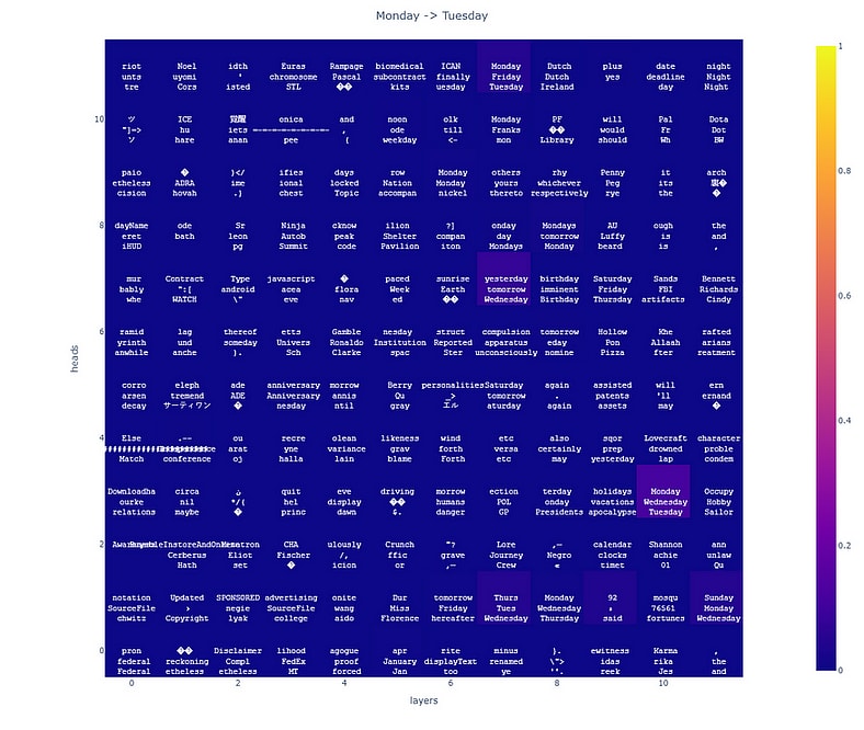
And the results for other prompts can be found here. A brighter cell colour represents a larger probability for the correct answer at that head.
Some observations:
We see that (10, 3) predicts the subject day as its most confident prediction for all tasks except for ‘Tuesday → Wednesday’, where it gets the correct answer.
(8, 1) is good at predicting days, but not necessarily the correct day.
(9, 1) occasionally predicts the correct day in its top 3, but with other seemingly irrelevant tokens.
Which heads are able to push the correct day highly? A good metric for this may be looking at which heads can predict the correct day above all other days, without concerning ourselves with how strong these predictions are compared to all other non-day tokens. Running such a script tells us that the only head that has this behaviour is (9, 1).
Behaviour of (10, 3)
How is (10, 3) useful for the task? Concretely,
Is (10, 3) a copying head?
Why would such a behaviour be useful?
Are there any other copying heads?
If we apply the logit lens technique (but ignoring top token predictions) and see the probs for the subject day of each prompt, we get
As expected, (10, 3) has a strong probability towards the subject day, with a mean prob of 0.5869, but (6, 9) is typically pushing with an even greater strength, with a mean prob of 0.8075! We also see that (7, 10) and (8, 1) have similar behaviours, with probs 0.4078 and 0.5489 respectively. A copying behaviour, and therefore these heads, may be useful for propagating the context of the task throughout the model, so these should be remembered for our in-vitro experiments.
Behaviour of (9, 1)
In this section, we claim that (9, 1)’s operation is that it is applying the ‘algorithm’ of next day prediction given sufficient context, i.e. it is directly incrementing the subject day to the next day. This is reasonable as it is the unique head to push the correct day over all other days consistently across all tasks, but we also see that some seemingly irrelevant tokens are present in its top tokens.
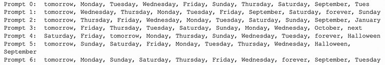
Looking in more detail at (9, 1)’s top token predictions, we see that its top 10 tokens (separated by a comma) across the prompts look like:
Sometimes it pushes the correct day without a space at the beginning, but overall it has the right idea. This tells us that (9, 1) cannot do everything on its own; it needs some way of removing the irrelevant tokens.
Its day distribution table looks like:
We can see that the diagonal below the main diagonal has a notably increased strength compared to the other days, corresponding to its pushing of the correct day above the rest.
A question now would be: how much input context does (9, 1) need to perform this prediction? It turns out to be very little, as we will see in the in-vitro experiments.
Attention patterns
We briefly take a look at the attention patterns of (9, 1) and (10, 3).
For (9, 1) and (10, 3) we see that:
Wrt. the final residual stream (the stream at which we are making a prediction of the next day), we can see that (10, 3) is strongly attending to the 4th token, i.e. the subject day, with attention 0.7133, which is expected as (10, 3) is a strong copier of this day. However, (9, 1) only slightly attends to the subject day with average attention 0.2097 and instead strongly attends to the BOS (beginning of sentence) token. Is the BOS token actually useful for (9, 1)’s operation?
We can try ablating the attention pattern of (9, 1), setting the attention for the 4th stream to 1 wrt. the final stream, resulting in the following attention pattern:
And at the end of the model the correct probs are:
An improved performance compared to the normal results!
It also turns out that just this 4th stream is uniquely sufficient among all other streams for (9, 1) and (10, 3). If we try setting each stream’s attention to 1 and the others to 0 wrt. the final stream, we get the average correct probs:
where the leftmost bar is the average correct prob in normal conditions. So allowing the heads to focus solely on the subject stream is highly beneficial to performance and other streams seem not helpful.
So the high attention towards the BOS token could be a bit of a blunder by the model. But what exactly is the 4th stream providing to the heads?
The top 10 tokens for the 4th stream input to (9, 1) look like:
And for (10, 3) they look like:
This echoes previous results (Geva et al., 2022) on the interpretability of MLP outputs to attention head outputs: these promote semantically similar outputs in the residual stream.
Both heads have very similar inputs. The subject day never appears in the top 10 tokens, and so the heads must be obtaining task context by some other representational means. Situations like this may be examples of where logit lens are ineffective: the goal here may be forming a certain representation to be used by the heads, as opposed to passing it specific, interpretable token representations like days.
Logit lens applied to layers
Our above analysis concerns the behaviour of heads, but it is also necessary to understand what is going on at a higher level, such as what layers are outputting. This will give us a wider view as to how the 12 heads of each layer are coming together to form useful representations. We apply logit lens at the very end of each layer to get the following:
This gives a clearer picture of how the predictions develop across the layers. Some things:
The probability for the correct day (brighter colour means higher) is actually maximal at the end of layer 10, not at the end of layer 11 as you would expect. We could therefore see layer 11 as being destructive for the task.
The 8th and 9th layers have “ tomorrow” as the top token (for all except 1 task), and this is removed by the end of layer 10. Is this token useful in some way, or is it irrelevant? If irrelevant, could this be why the copying behaviour of (10, 3) is useful? To get rid of such irrelevant tokens by pushing day tokens above them?
Except for the ‘Monday → Tuesday’ task, the correct day is above all other days at the end of layer 9. At layer 8 however, the subject day is above all the other days.
Looking at the inputs to layer 9 and 10 at the last stream in more depth, we see that layer 9 has top 10 tokens:
And layer 10 has:
It makes intuitive sense that a good context for the heads to operate in would be this kind of ‘temporal’ context, with the concepts of days, months and time.
But is the “ tomorrow” token actually useful? We try adjusting the logits for “ tomorrow” by adding a multiple α of “ tomorrow”’s unembedding vector to the residual stream at the end of layer 8. If we pick α = −1, we get a decrease in correct probs:
but also a decrease in the attention to the 4th stream at (9, 1) compared to normal conditions, now with average attention 0.1522. With α = −5 there is an even greater drop in correct probs:
and the average attention is now 0.03221.
At the opposite end, picking α = 5 gives average attention 0.5864, and the extreme of α = 100 gives average attention 0.7499.
This displays why the “tomorrow” token is useful: it increases the 4th stream attention, and we have evidence that this is a very useful stream for (9, 1).
Layer MLPs
What is the role of layer MLPs? One way to measure the effect of a layer’s MLP is to apply logit lens before and after the MLP output is added to the stream (see layer diagram in Model Structure section) and observe the correct prob. Plotting the difference in correct prob before and after the MLP (higher value means a higher prob after the MLP) looks like:
where we have averaged across the prompts. And so it can be seen that layer 9’s MLP seems the most helpful towards directly pushing the correct day, and that layer 7’s MLP seems the most destructive in doing so. Looking closer at the layer 9 MLP, we see that the day distribution before and after looks like:
There is a noticeable movement of logits from the diagonal to below the diagonal, and so we theorise that the layer 9 MLP is a decopying MLP, with the main purpose of decreasing the logits of the subject day. This behaviour could have been learnt in order to account for the overprediction of subject information by heads with copying behaviours. This evidence that the layer 9 MLP is good at decopying will be useful later in our in-vitro experiments.
The above measure can be seen as a ‘local’ method as we are unembedding inside the model at each individual layer. We can also consider a more ‘global’ measure of layer behaviour by zero ablating each MLP component and observing the resultant effect on the final output at the end of the model. Carrying out such a procedure and computing the difference in prob compared to normal conditions (lower value means lower prob after disabling MLP) gives:
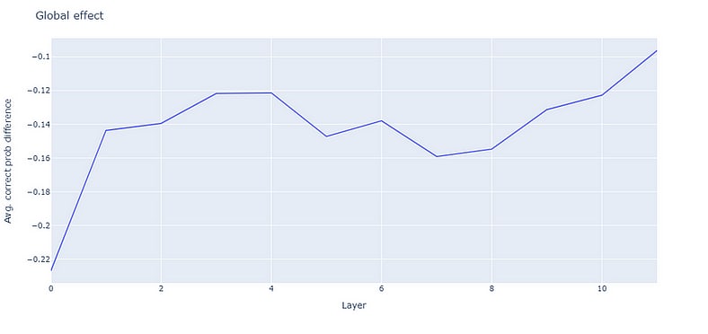
We see that globally, disabling the layer 0 MLP has the greatest negative effect on performance by a significant margin. Similarly, this MLP will also arise in the in-vitro results as being important for a minimal circuit.
Closing remarks
From these results, the key insights are:
(9, 1) can uniquely push the correct day above the other days.
(10, 3) exhibits copying behaviour and its ablation has significant negative impact.
(9, 1) and (10, 3) seem to only require the subject input stream, specifically the 4th stream, for their operation.
MLP 9 decopies, and ablating MLP 0 has significant negative impact.
In-Vitro Results
Introduction
Our in-vivo results have given a good idea as to what certain heads do and which seem the most important. The purpose of this section is to now test some theories based on these results in ‘in-vitro’ environments, reducing the model to a small subset of fundamental heads and studying them in isolation.
Finding a subset under mean ablation
(this section has been shortened, but more details can be found here)
We end up finding that even under mean ablation of everything except the heads [(9, 1), (10, 3)], the top tokens of these two heads (found via logit lens) are near identical to the top tokens with no ablation at all (as seen in in-vivo experiments), implying that the incoming context at the 4th stream is not destroyed under this ablation. However, these two heads are still insufficient for good correct probs because the context at the final stream incoming to layer 9 and 10 is destructive due to the significant ablation, as the results of the heads are added to the layer inputs residually. As a result, the useful information from the heads is destroyed.
To amend this, we add some heads from layer 8, and find that mean ablating everything except [(8, 1), (8, 6), (8, 8), (9, 1), (10, 3)] has, at the end of layer 10, correct probs:
providing some evidence that (8, 1), (8, 6), and (8, 8) were successful in building layer input context such that the residual connection is no longer destructive.
These results involve mean ablating most of the model — the weakest form of ablation we’ve defined — and so a question is how does the model behave under a stricter form of ablation? We now explore this.
Finding a subset under random ablation
(this section has been shortened, but more details can be found here)
We find that under random ablation of everything except [(9, 1), (10, 3)], the top tokens for these two heads are again very similar to the top tokens under no ablation at all. Our previously found set of 5 heads does not work too well under random ablation, but if we add a copying head like (6, 9) (to remember task context), we get that at the end of layer 10, the correct probs are:
The main point all of this emphasises is that the heads (9, 1) and (10, 3) can perform their individual operations under very little context (as seen by their top tokens remaining invariant), but we must include other heads to prevent destruction of their info.
How about we approach the problem from a different perspective and try to suppress this residual connection by some means and see if (9, 1) and (10, 3) alone can complete the task? We now explore such ideas.
Testing our theories
Given all this data, we can now start testing some theories more deeply. Particularly, we see that (9, 1) and (10, 3) can operate fine on an individual level with little context, however the final output of the model is bad due to the residual connection between the original layer input and the head outputs.
One way of further verifying this would be to somehow suppress this residual connection and to then observe a good performance. A setup capable of this could be the following:
Note that this suppresses the residual connection as the output from layers 0 to 8 are not added back to the head outputs. Only the head outputs are added together, and then unembedded. Running this and finding the correct probs of the output Y gives correct probs:
Though the final task fails, the other tasks are quite high given the little context being provided. The average attention patterns look like:
Note that the attention patterns look similar to the in-vivo patterns we found.
The above result is some strong evidence towards the theory that the residual connection is destructive and the heads require little context. But can we remove even more context? The same setup, but instead zero ablating everything from layer 0 to layer 8, gives correct probs:
Really not great. The average attention patterns here look like:
Unlike in the random ablation case, the attention has been completely destroyed. Is this the main reason for the collapse in performance? We can ablate the attention pattern of (9, 1) and (10, 3) such that the attention of the 4th stream is 1 wrt. the final stream. This gives correct probs:
A substantial improvement, supporting the theory that the attention towards the 4th stream is detrimental for performance. Overall, this setup looks like:
With this new setup of mostly zero ablation and intervened attention, what’s really happening to the token embeddings? Since no heads in the ablated layers have any contribution to the residual stream, the original token embeddings are just passing through the MLPs for each layer and being added back to the stream residually. We saw that the layer 0 MLP seemed important globally. How about providing (9, 1) and (10, 3) with just the output from layer 0 with its heads zero ablated? This gives correct probs:
Overall this gives the setup:
Probabilities are useful, but what are the top token predictions for this setup?
Prompt 0 fails as it predicts Tuesday without the space, and prompt 6 fails as the subject day logits are too high. The day distribution for the final output of the setup looks like:
The diagonal has quite strong logits, so perhaps the copying behaviour of (10, 3) is too strong? We have found that the layer 9 MLP is good at decopying, so it could be useful here. Including the layer 9 MLP in the setup like so:
gives correct probs:
now giving the correct answer for all prompts.
Generalizations
Introduction
We’ve seen that an extremely simple circuit of 2 heads and 2 MLPs are capable of completing the task of next day prediction. Specifically, (9, 1) is able to find the next day among all 7 days, and the other components (2 MLPs and (10, 3)) are necessary to provide context, to decopy, and to remove irrelevant tokens produced by (9, 1). But perhaps this is too fine tuned to the task and does not provide useful mechanistic knowledge? This section touches on more general capabilities of the involved components.
The month task
The month task is very similar to the day task we are used to, except we now try to predict the next month given prompts of the form:
where similarly to the day task, <month> is a placeholder for one of the 12 months: “January”, …, “December”.
We first check how the model does on this task in normal conditions. It achieves correct probs of:
We can also run a similar script that found (9, 1) in the day task, but instead finds heads that can push the correct month more than the other months consistently for all 12 prompts. Such a script returns:
[]
I guess this task is a bit more difficult; no heads are capable of such a behaviour. But if we run the same script except we allow it to be wrong for just a single prompt out of the 12, we get:
[(9, 1)]
We now try the found setup on this task, but with the attention of the 5th stream (the month token) set to 1 wrt. the final stream, and observe correct probs:
Almost perfectly solving the task, except for “July → August” where it predicts “ Aug” instead. This task was not even considered during the formation of the found setup, so the fact that it performs extremely well on this new task is surprising.
We see that in this setup, (9, 1) has top 10 tokens:
And (10, 3) has top 10 tokens:
The behaviour of (9, 1) is less clear here: sometimes the correct month does show up, but it is much more inconsistent compared to the day task. (10, 3) however still maintains its copying behaviour. Under this setup, the ‘day’ distribution (though now of course it is for months) for (9, 1) and (10, 3) look like:
Resembling the distributions for the day task.
The number task
So it turns out that (9, 1) can pick the successor of an individual day and month. Does this generalise even further? What about numbers?
We now try the task:
where <num> is a placeholder for a natural number up to some chosen n: “1”, “2”, …, “{n}”
The model in normal conditions does surprisingly bad. For example for n = 10 we have correct probs:
And for larger n the probabilities further decay to zero. We try the very simple setup of:
where note we have now set the 2nd stream attention to 1 wrt. the final stream, as the 2nd stream corresponds to the subject number. We see a significant improvement in performance, where for n = 10 the correct probs are:
And even for n = 100, we see an average correct prob of 0.7363… with 83⁄100 of the prompts answered correctly.
In this task, (9, 1) is very confident in its predictions and produces no irrelevant tokens (text involving numbers were much more common in the training data than text involving days/months?) and so the usual jobs of (10, 3) and MLP 9 refining (9, 1)’s answer seem to not be needed.
Final remarks
Say our task has a subject token at token index . For example, in the day task and in the number task .
If for head we ablate the attention of the th stream to 1 wrt. the final stream, the output of the head at the final stream is:
where is the input to at the th stream.
Now focusing on (9, 1), we can define such that under the above attention ablation, the output of (9, 1) at the last stream is simply:
In this description, we have reduced the ‘successor’ operation of (9, 1) to a single, low-rank square matrix . An interesting question is whether this matrix is interpretable and how does it operate? How is it utilising the th stream context? Is it taking advantage of a geometric relationship between tokens (something similar to a rotation from one token to the next), or something else? How much further does its capability generalise?
Closing remarks
Through the use of various techniques and heuristics, we have been able to discover a simple circuit that is capable of solving the day task, and have found that the components of this circuit generalise outside of the task for which it was found. We saw that two heads were capable of performing important roles, but the difficulty was in supplying these heads with the right context for them to do their job.
If we wish to apply a language model to a specialised task, it’s possible that the model may not perform well/fail (as seen in the number task) but that there exists a small (and therefore more manageable) circuit within the model that is very capable of the task now that other components which are not helpful/introduce noise are removed.
The most intriguing component we found was the head (9, 1); it can apply a ‘successor’ algorithm in various contexts. The mechanism of how this algorithm operates is not known, and has not been explored in much depth, however understanding this may provide insights into the generality of behaviours that are capable of being learnt by language models.
Appendix
Notation
| is a tensor with . | |
| The batch size of the input. | |
| The sequence length of the input (including BOS token). | |
| The dimension of the residual stream. For GPT-2 small this is 768. | |
| The vocab size of the model. For GPT-2 small this is 50,257. | |
| The number of layers in the model. For GPT-2 small this is 12. | |
| The number of heads per layer. For GPT-2 small this is 12. | |
| head | The th head of the th layer. |
| The dimensionality of query, key and value vectors inside a head (see below). For GPT-2 small this is 64. | |
| The query matrix for head , of shape | |
| The key matrix for head , of shape | |
| The value matrix for head , of shape |
Resources
For those new to transformer models and mechanistic interpretability, we briefly provide a (certainly) non-exhaustive list of resources to help get started!
If you just want to play with GPT-2, check out this online demo or Hugging Face GPT-2.
The Illustrated GPT-2 (Visualizing Transformer Language Models), Jay Alammar — a great introduction to transformer models with plenty of accompanying diagrams.
A Mathematical Framework for Transformer Circuits, Anthropic — the next step to getting to grips with transformers (complete with a problem set to test your understanding).
Resources from Neel Nanda, particularly:
- TransformerLens and links therein
- his YouTube playlist on ‘What is a Transformer?’
- Mechanistic Interpretability Quickstart Guide
- A Comprehensive Mechanistic Interpretability Explainer & GlossaryThe work of companies like Anthropic or Redwood Research.
I sometimes see posts like this that I can’t follow in depth due to insufficient math ability, but skimming them they seem important-if-true so I upvote them anyway. I do want to encourage stuff like this but I’m concerned about adding noise through not-fully-informed voting. Would it be preferable to only vote on things I understand better?
I don’t understand why this comment has negative “agreement karma”. What do people mean by disagreeing with it? Do they mean to answer the question with “no”?
Note that this behavior generalizes far beyond GPT-2 Small head 9.1. We wrote a paper and a easier-to-digest tweet thread
I think these are top 10 tokens.
I always feel happy when I read alignment posts I don’t understand, for some reason.
Upon rereading to find where I didn’t understand, I found I didn’t lose much of the text, and all I had previously lost was unimportant.
My happiness is less, but knowing feels better.