Features and Adversaries in MemoryDT
Keywords: Mechanistic Interpretability, Adversarial Examples, GridWorlds, Activation Engineering
This is part 2 of A Mechanistic Interpretability Analysis of a GridWorld Agent Simulator
Links: Repository, Model/Training, Task.
Epistemic status: I think the basic results are pretty solid, but I’m less sure about how these results relate to broader phenomena such as superposition or other modalities such as language models. I’ve erred on the side of discussing connections with other investigations to make it more obvious how gridworld decision transformers may be useful.
TLDR
We analyse the embedding space of a gridworld decision transformer, showing that it has developed an extensive structure that reflects the properties of the model, the gridworld environment and the task. We can identify linear feature representations for task-relevant concepts and show the distribution of these features in the embedding space. We use these insights to predict several adversarial inputs (observations with “distractor” items) that trick the model about what it is seeing. We show that these adversaries work as effectively as changing the feature (in the environment). However, we can also intervene directly on the underlying linear feature representation to achieve the same effects. Whilst methodologically simple, this analysis shows that mechanistic investigation of gridworld models is tractable and touches on many different areas of fundamental mechanistic interpretability research and its application to AI alignment.
We recommend reading the following sections for readers short on time:
Read the Introduction sections on the task and observation embeddings.
Read the section describing extraction of the instruction feature via pca.
Read the results sections describing using adversaries to change the instruction feature and comparing adversaries to direct intervention.
Key Results
Object Level Results
We show that our observation space has extensive geometric structure.
We think this structure is induced by properties of experimental set up (partial observations), architectural design (compositional embedding schema) and the nature of the specific RL task.
The learned structure included the use of clustered embeddings and antipodal pairs.
We see examples of isotropic and anisotropic superposition.
We identify interpretable linear feature representations in MemoryDT’s observation embedding space.
We find that Principal Component Analysis of a subset of embedding vectors produces vectors that linearly classify the input space according to task relevant concepts.
We find underlying linear feature representations appear “smeared” across many embeddings which we interpret as a particularly simple form of equivariance.
We causally validate one of these features, the “instruction feature”, using adversarial inputs/embedding arithmetic and direct interventions.
It’s easy to break models trained on simple tasks, but our adversaries are targeted, directly flipping the models’ detection of the learned feature.
The prediction behind our adversaries also included an arithmetic component which we validated, enabling us to relate our results to arithmetic techniques used to generate steering vectors.
For rigour and completeness, we use direct intervention on the feature to show that it is causal.
Lastly, we confirm that the adversarial inputs transfer to a different model trained on the same data indicating consistent with our adversary working via a feature not a bug.
Broader Connections
While this post summarises relatively few experiments on just one model, we find our results connect with many other ideas which go beyond the details of just this model.
We observe superposition in a gridworld model juxtaposing previous results in toy models and language models.
We show that interpretability techniques can be used to predict effective adversaries that generalise and hypothesise possible mechanisms behind adversarial attacks on language models.
We add to a body of evidence suggesting that it’s possible to find and intervene on linear feature representations, showing that they exist and are causal.
We relate our observations to the phenomenology of steering vectors.
Introduction
Why study GridWorld Decision Transformers?
Decision Transformers are a form of offline RL (reinforcement learning) that enables us to use Transformers to solve traditional RL tasks. While traditional “online” RL trains a model to receive reward by completing a task, offline RL is analogous to language model training with the model being rewarded for predicting the next token.
Decision Transformers are trained on recorded trajectories which are labelled with the reward achieved, Reward-to-Go (RTG). RTG is the time-discounted reward stream that the agent should be getting, i.e. if it’s set close to 1 then the model will be incentivised to do well because it will be taking actions consistent with the reference class of other agents that got this reward. RTG isn’t critical to this post but will be discussed in more detail in subsequent posts.
We’re interested in gridworld decision transformers for the following reasons.
Decision Transformers are smaller/simpler than the language models we want to understand and align. Decision Transformers are transformers, the training trajectories operate a lot like a training corpus and RTG works a lot like an instruction/goal prompting. It may be the case that various phenomena associated with large language models are also present in these models and can be studied.
We might be able to study alignment-relevant phenomena in decision transformers. Previous work has studied alignment-relevant phenomena (such as goal misgeneralization) in the absence of interpretability, or with non-transformer architectures. Decision transformers are more analogous to pre-trained language models or instruction-tuned language models by default, but we could conceivably train them with online learning analogous to RLHF.
We’re working with gridworld tasks because they’re simpler and easier to write. Gridworld RL tasks have been used to study alignment-relevant properties in the past and we’re able to avoid training convolutional layers to process images which speeds up training.
AI Alignment and the Linear Representation Hypothesis
The linear representation hypothesis proposes that the neural networks represent features of the input as directions in latent space.
This post focuses on linear representations for 3 reasons:
The Linear Representation Hypothesis seems likely to be true. Evidence on many fronts suggests that some version of the linear representation hypothesis holds. Also, recent publications show evidence that is possible to find and interpret linear representations in the residual stream. Therefore, it’s likely that MemoryDT and other gridworld / decision transformers will make use of linear representations.
The Linear Representation Hypothesis seems likely to be useful. If the linear representation hypothesis is true and we’re able to find the corresponding directions in deep neural networks, then we may be able to read the thoughts of AI systems directly.Such a feat would not only be step one in retargeting the search but also a huge win for interpretability and many other alignment agendas. Showing that we can retarget the search on MemoryDT is one of the various win scenarios for our work.
Our results seem interesting from the perspective of superposition, a phenomenon that represents a significant obstacle to interpretability. Previously, it was thought that finding meaningful directions in a residual stream would be very difficult due to superposition/entanglement (the property whereby linear features are represented in shared dimensions). Results from recent work with sparse autoencoders found interpretable features that clump together in groups (anisotropic superposition) as opposed to repelling and spreading as far as possible (isotropic superposition).
Diagram from Towards Monosemanticity: Decomposing Language Models With Dictionary Learning
The MiniGrid Memory Task
MemoryDT is trained to predict actions in trajectories produced by a policy that solves the MiniGrid Memory task. In this task, the agent is spawned next to an object (a ball or a key) and is rewarded for walking to the matching object at the end of the corridor. We refer to the first object as the “instruction” and the latter two objects as the “targets”.
Figure 1 shows all four variations of the environment. Please note:
The agent is always implicitly present at position (3,6), centred at the bottom of the image.
The action space is made up of the actions “Left”, “Right”, and “Forward”, along with four other actions not useful in this environment.
MemoryDT receives its observations in blocks of three tokens (R, S, A), with the action produced by the model and the Reward-to-Go and the next state/observation provided by the environment.

Figure 1: MiniGrid Memory Task Partial Observations. Above: All 4 Variations of the MiniGrid Memory Task as seen from the starting position. Below: A recording of high-performing trajectories.
This task is interesting for three reasons:
The optimal policy is well described as learning a simple underlying algorithm described by the boolean expression A XOR B. The optimal trajectory shown in Figure 1 involves walking forward four times and turning left or right, followed by forward. However, labelling the instruction and target as boolean variables, the optimal policy is to turn left if A XOR B and right otherwise. The XOR operation is particularly nice for interpretability since it is symmetric in A and B, and changing A or B will always change the correct decision. Therefore, all beliefs about the instruction/targets should be action-guiding.
Observations generated in this task include redundant, correlated and anti-correlated features, encouraging abstractions. The gridworld environment makes this true in many ways:
The target configuration is detectable via the left or right position alone and in any observation in which they are visible.
The presence of a key at a position implies the absence of a ball at the same position (hence, instructions/targets becoming binary variables).
Since the instruction does not change mid-episode, observations of the same object are redundant between observations.
A partially observable environment forces the use of the transformer’s context window. The optimal trajectory involves only seeing the instruction once, forcing the use of the context window. This is important since it adds complexity which justifies the use of a transformer, which we are interested in studying.
Figure 2 shows how the decision transformer architecture interacts with the gridworld observations and the central decision. We discuss tokenisation of the observation in the next section.
Figure 2: Decision Transformer Diagram with Gridworld Observations. R corresponds to the tokenised Reward-to-Go, and S stands in for state (replaced with O in practice; we have partial observations). A corresponds to action tokens.
MemoryDT Observation Embeddings are constructed via a Compositional Code.
To adapt the Decision Transformer architecture to gridworld tasks, we tokenise the observations using a compositional code whose components are “objects at (x,y)” or colour at (x,y). For example, Key at (2,3) will have its embedding, and so will Green (2,3), etc. Figure 3 shows example observations with important vocabulary items shown.
Figure 3. Example Observations with annotated target/instruction vocabulary items.
For each present vocabulary item, we learn an embedding vector. The token is then the sum of the embeddings for any present vocabulary items:
Where Ot is the observation embedding (which is a vector of length 256), i is the horizontal position, j is the vertical position, c is the channel (colour, object or state), and is the corresponding learned token embedding with the same dimension as the observation embedding. is an indicator function. For example, means that there is a key at position (2,6).
Figure 4 illustrates how the observation tokens are made of embeddings, which might themselves be made of features, which match the task-relevant concepts.
Figure 4: Diagram showing how concepts, features, vocabulary item embeddings and token embeddings are related. We learn embeddings for each vocabulary item, but the model can treat those independently or use them to represent other features if desired.
A few notes on this setup:
Our observation tokenisation method is intentionally linear and decomposable into embeddings (linear feature representations). Constructing it like this makes it harder for the model to memorise the observations since it must create them from a linear sum of fundamentally (more) generalising features. Furthermore, the function A XOR B can’t be solved using a linear classifier, stopping the model from solving the entire task in the first observation.
Our observation tokenisation method is compositional with respect to vocabulary items but not task-relevant concepts. The underlying “instruction feature” isn’t a member of the vocabulary.
The task-relevant concepts have a many-to-many relationship with vocabulary items. There are different positions from which the instruction/targets might be seen.
Some vocabulary items are much more important for predicting the optimal action than others. Keys/Balls are more important, especially at positions from which the instruction/targets are visible.
Vocabulary item embeddings will have lots of correlation structure due to partial observability of the environment.
Results
Geometric Structure in Embedding Space
To determine whether MemoryDT has learned to represent the underlying task-relevant concepts, we start by looking at the observation embedding space.
Many embeddings have much larger L2 norms than others.
Channels likely to be activated and likely to be important to the task, such as keys/balls, appeared to have the largest norms, along with “green” and other channels that may encode useful information. Some of the largest embedding vectors corresponded to vocabulary items that were understandable and important, such as Ball (2,6), the ball as seen from the starting position, whilst others were less obvious, Ball (0,6), which shouldn’t appear unless the agent moves the ball (it can do that). Embedding vectors are initialised with l2 norms of approximately 0.32, but these vectors weren’t subject to weight decay, and some grew during training.
Figure 5: Strip Plot of L2 Norms of embedding vectors in MemoryDT’s Observation Space.
Cosine Similarity Heatmaps Reveal Geometric Structure
We initially attempted PCA / U-Map for dimensionality reduction, however, neither was particularly informative. However, we were able to borrow the concept of a clustergram from systems biology. The idea is to plot a heatmap of the adjacency matrix, in this case, the cosine similarity matrix of the embeddings and reorder rows according to a clustering algorithm. The resulting cosine similarity heatmaps (methods) were interesting with and without the reordering of rows for clustering (Figure 6).
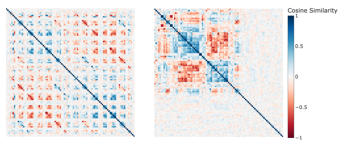
Figure 6: Cosine Similarity Heatmap of Embeddings for Key/Ball Channels. LHS: The order of rows/columns is determined by descending order given channel, y-position, x-position. The first row is Key (0,0), the next is Key (0,1) and so forth. RHS: The order of rows/columns is determined by agglomerative clustering. Figure 6 is best understood via interactions (zooming/panning).
There were a number of possible stories which might explain the structural features observed in Figure 6. Many embeddings don’t have very high cosine similarity with any others. These embeddings with low norms weren’t updated much during training.
Two effects may be interpreted with respect to correlation or anti-correlation:
Spatial Exclusivity/Anti-correlation was associated with antipodality: Without reordering, we can see off-centre lines of negative cosine similarity, which correspond to keys/balls at the same positions. This may suggest that the mutual exclusivity of keys/balls at the same position induced anti-correlation, which led to antipodality in these representations, consistent with results in toy models.
Correlated Vocabulary items had higher cosine similarity: Some vocabulary items have particularly high cosine similarity. For example, vocabulary items associated with one variation of the target configuration are seen from the starting position: key (1,2) and ball (5,2).
To address these ideas more directly, we plotted cosine similarity to determine whether the two vocabulary items shared the same channel (key or ball) or position (Figure 7).
Figure 7: Distribution of Cosine Similarity of pairs of embeddings/vocabulary items (limited to Key/Ball channels), filtered to have an L2 norm above 0.8.
Even though channel/position is not a perfect proxy for correlation beyond the anti-correlation induced by spatial exclusivity, Figure 7 shows some general trends better than Figure 6. Beyond potentially interesting trends (which aren’t trivial to interpret), we can see many outliers whose embedding directions relative to each other can’t easily be interpreted without reference to the training distribution.
This leads us to hypothesise that semantic similarity may also affect geometric structure. By “semantic similarity”, we mean that some vocabulary items may be related not just by when they are likely to occur but by the actions that the decision transformer should make having observed them. To provide evidence for such a hypothesis, we focus on groups of vocabulary items with particularly absolute cosine similarity and clusters. For example, we observed clusters corresponding to vocabulary items in a single channel at multiple positions, such as Keys at (0,5), (2,6) and (4,2). Interpreting these clusters was possible with reference to the training distribution, specifically looking at which positions the agent might be in when those channels are activated (Figure 8).
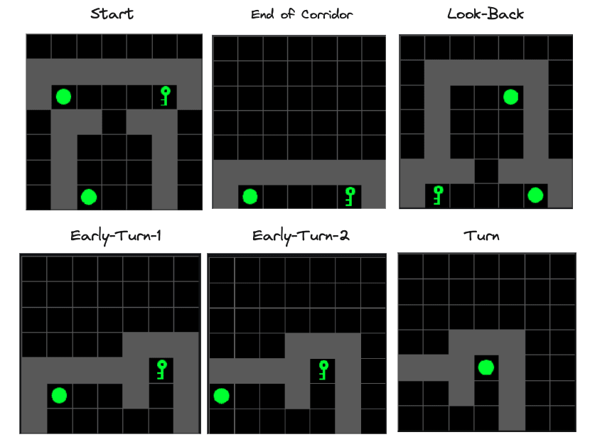
Figure 8: Reference Observations to assist interpretation of Feature Maps. The agent is always in position (3,6).
By combining the clusters observed in Figure 8 with the distribution of possible observations in the training dataset, it’s possible to see several semantically interpretable groups:
Targets seen from the end-of-corridor and the “look-back” position. These included Keys and Balls at (1,6) and (5,6).
Targets, as seen from the start. These included Keys and Balls at (1,2) and (5,2).
Instructions as seen from various positions: These include: Start → (2,6), Look-Back → (4,2) (4,3). Early Turn 1, 2 → (1,5), (0,5).
At this point, we hypothesised that each of these vocabulary items may contain underlying linear features corresponding to the semantic interpretation of the group.
Extracting and Interpreting Feature Directions in MemoryDT’s Observation Embeddings
To extract each feature direction, we perform feature extraction via Principal Component Analysis on the subset of relevant embedding vectors. Using PCA, we hope to throw away unimportant directions while quantifying the variance explained by the first few directions. We can attempt to interpret both the resulting geometry of the PCA and the principal component directions themselves. (see methods).
To interpret the principal component directions, we show heatmaps of the dot product between the PC and each embedding vector, arranging these values to match the corresponding positions in the visualisations of gridworld partial observations. These heatmaps, which I call “feature maps”, have much in common with heatmaps of convolutional layers in vision models and represent virtual weights between each embedding the underlying principal component. (see methods).
The Primary Instruction Feature
Figure 9: Exploratory Analysis of the “Instruction” subset of Observation Embeddings.
Left) Cosine Similarity Heatmap of the Instruction Embeddings.
Right) 2D Scatter Plot of the first 2 Principal Components of a PCA generated from the embedding subset.
Previously, we identified keys/balls at positions (4,2), (4,3), (0,5) and (2,6) as clustering and hypothesised that this may be due to an underlying “instruction feature”. The first two principal components of the PCA explain 85.12% of the variance in those embeddings and the first two dimensions create a space in which keys/balls appear in antipodal pairs (Figure 9). This projection is reminiscent of both feature splitting/anisotropic superposition (which is thought to occur when highly correlated features have similar output actions) and antipodality found in toy models.
PC1 separates keys from balls independently of position, making it a candidate for a linear representation of an instruction feature. One way to interpret this is a very simple form of equivariance, where the model detects the instruction at many different positions as the instruction.
To visualise this instruction feature, we generate a feature map for PC1 (Figure 10), which shows that this feature is present to varying degrees in embeddings for keys/balls at many different positions where the instruction might be seen. We note that the instruction feature tends to be present at similar absolute values but opposite signs between keys and balls, suggesting a broader symmetry in the instruction feature between keys and balls.
Figure 10: Feature Map showing Instruction PC1 Values for all embeddings corresponding to Keys/Ball.
Another Instruction Feature?
PC2 in the Instruction subset PCA is less easy to interpret. Figure 9 distinguishes whether the instruction has been identified from “look-back” and “starting” positions. However, it appears to “flip” the effect it has for embeddings, which correspond to “instruction is key” vs “instruction is ball”. Moreover, the feature map for PC2 (Figure 11) shows keys and balls at (3,4) as having noticeable cosine similarity with this direction, which doesn’t fit that interpretation. Nor does this explanation predict that keys/balls at (4,3), a position similar to the look-back feature, barely projects onto PC2.
We suspect that PCA fails at finding a second interpretable feature direction because it finds orthogonal directions, however, it’s not obvious that there isn’t a meaningful underlying feature. We plan to investigate this further in the future.
Figure 11: Feature Map showing Instruction PC2 Values for all embeddings corresponding to Keys/Ball.
Target Features
Figure 12: Exploratory Analysis of the Target Embeddings. Left) Cosine Similarity Heatmap of the Target Embeddings. Right) 2D Scatter Plot of the first 2 Principal Components.
For the target feature, we identified two separate clusters, each made up of two sets of almost antipodal pairs (Figure 12). The geometry here is much closer to isotropic superposition/toy model results. The faint-checkerboard pattern suggests the slightest hint of a more general target feature, which we suspect may be learned if we trained MemoryDT for long enough.
The first two principal components of the resulting PCA explain 83.69% of the variance in those embeddings and produced interpretable feature maps (Figure 13):
Starting Target Feature: PC1 can be interpreted as reflecting the configuration of the targets as seen from the starting position (1,2) and (5,2). There’s slight evidence that targets are seen at intermediate positions while walking up to the targets (1,3) and (1,4).
End Target Feature: PC2 can be interpreted as reflecting the configuration of the targets as seen from the end of the corridor position (1,2) and (5,2).
Figure 13: Feature map showing Instruction PC1 Values (above) and PC2 embedding (below) for all embeddings corresponding to Keys/Ball.
Using Embedding Arithmetic to Reverse Detected Features
Embedding Arithmetic with the Instruction Feature
We previously observed that the group of vocabulary items associated with the instruction concept were separated cleanly into Keys and Balls by a single principal component explaining 60% of the total variance associated with the 6 vectors included. From this, we hypothesised that this principal component reflects an underlying “instruction feature”. To validate this interpretation, we want to show that we can leverage this prediction in non-trivial ways such as by generating feature-level adversaries (as previously applied to factors found via dictionary learning in language models and copy/paste attacks in image models)
Based on the previous result, we predicted that if we added two vocabulary items matching the opposite instruction (ie: if the instruction is a key, seen at (2,6), we can add a ball to (0,5) and a ball to (4,2)) and this would induce the model to behave as if the instruction were flipped. I’ve drawn a diagram below to explain the concept (Figure 14).
Figure 14: Diagram showing the basic inspiration behind “instruction adversaries”.
Effectiveness of Instruction Feature Adversaries
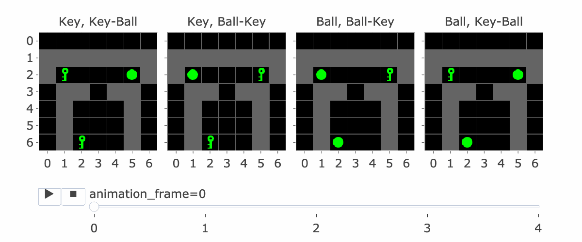
Figure 15: Animation showing the trajectory associated with the Instruction Reversal Experiment.
To test the adversarial features / embedding arithmetic hypothesis, we generated a set of prompts/trajectories ending in a position where the model’s action preference is directly determined by observing the instruction being a key/ball (Figure 15). For each of the target/instruction configurations in Figure 15, we generate five different edits (Figure 14) to the first frame:
The original first frame:This is our negative control.
The first frame with the instruction flipped: This is our positive control. Changing the instruction from a key to a ball or vice versa at the first frame makes the model flip its left/right preference.
The first frame with the complement instruction added at (0,5). We expect this to reduce the left-right preference but not flip it entirely. (Unless we also removed the original instruction).
The first frame with the complement instruction added at (2,4). Same as the previous one.
The first frame with the complement instruction added at (0,5) and (2,4). Even though this frame was not present in the training data, we expect it to override the detection of the original instruction.
Note that due to the tokenisation of the observation, we can think of adding these vocabulary items to the input as adding adversarial features.
Note: I’m using the word “complement” because if the original instruction was a key, add a ball to reverse it and vice versa.
Figure 16: Adversarial Observation Token Variations. Added objects are shown in red though only the object embedding is added.
Figure 17 shows us the restored logit difference for each of the three test cases Complement (0,5), Complement (4,2) and Complement (0,5), (4,2) using the original frame as our negative control or “clean” input and Instruction Flipped as our “corrupt”/positive control.
Figure 17: Restored Logit Difference between left/right for instruction feature adversaries in “scenario 1”(MemoryDT). 8 facet images correspond to each target, instruction and RTG combination. (RTG = 0.892 corresponds to the highest possible reward that an optimal policy would receive. RTG = 0 corresponds to no reward, often achieved by going to the wrong target)
These results are quite exciting! We were able to predict very particular adversaries in the training data that would cause the model to behave (almost) as if it had seen the opposite instruction and did so from the feature map (an interpretability tool).
Let’s break the results in Figure 17 down further:
Adding two decoys isn’t as effective as reversing the original instruction. We expected that adding two “decoy” instructions would work as well as flipping the original instruction but the best result attained is 0.92 and most results are around 0.80-0.90.
Adding a single decoy isn’t consistently additive. If the effects were linear, we would expect that adding each single decoy would restore ~half the logit difference. This appears to be roughly the case half the time. If the effect was non-linear and we needed both to achieve the result, adding each alone would achieve a negligible effect. This also happens in some cases.
The effect of individual decoys should be symmetric in their effects under our theory but they aren’t always. In the case of Ball, Ball-Key at RTG 0. Adding a key at (0,5) alone achieves 0.43 of the logit difference of both complements but adding a key at (4,2) achieves 0.03.
Proving that Instruction Feature Adversaries operate only via the Instruction Feature.
Whilst the previous results are encouraging, we would like to provide stronger evidence behind the notion that the projection of the embedding space into instruction feature direction is causally responsible for changing the output logits. To show this we provide two lines of evidence:
We show that the adversarial inputs are genuinely changing the presence of the instruction feature.
We show that we can directly intervene on the instruction feature to induce the same effects as the adversaries or flip the instruction.
The adversarial inputs are changing the presence of the instruction feature.
For each of the forward passes in the experiment above, we plot the dot product of the instruction feature with the observation embedding against the difference between the logits for turning left and right (Figure 16). We see that:
We weren’t flipping the instruction feature hard enough. Complement (0,5), (4,2) isn’t projecting as strongly into the instruction feature direction as the Instruction Flipped observation. This may explain why our restored logit differences weren’t stronger before.
MemoryDT doesn’t implement “A XOR B”. Flipping the sign on the instruction feature often flips the action preference. However, it fails to do so when the target configuration is “Key-Ball” and RTG = 0.892. MemoryDT mostly wants to predict “A XOR B” at high RTG and its complement at low RTG, but it doesn’t quite do this.
It’s unclear if logit difference is a linear function of A, suggesting heterogeneous mechanisms. For example, some scenarios appear almost sigmoidal (Ball, Ball-Key at RTG = 0.892). Others might be linear (Key, Key-Ball at RTG = 0.0). If the underlying functional mappings from feature to logit difference differed, this may suggest different underlying mechanisms.
Figure 18: Measuring the projection of the first frame observation embeddings into the Instruction PC0 direction (x-axis) and showing the logit difference between left/right (y-axis).
Direct Interventions on the Instruction Feature
We directly intervene on the instruction feature in each scenario tested above, again plotting the logit difference for the final left minus right direction (Figure 19).
This similarity in the functions mapped by the adversarial intervention (Figure 18) and the direct intervention is striking! They show a similar (and clearer) functional mapping from the instruction feature sign/magnitude to the logit difference, suggesting the instruction feature entirely explains our adversarial results.
Figure 19: Intervened Instruction PC0 direction (x-axis) and showing the logit difference between left/right (y-axis).
Do the Instruction Feature Adversaries Transfer?
Finally, since our explanation of the instruction feature suggests that it represents a meaningful property of the data and that our embedding arithmetic can be interpreted as adversaries, it is reasonable to test if those adversaries transfer to another model trained on the same data. MemoryDT-GatedMLP is a variant of MemoryDT that is vulnerable to the same adversarial features (Figure 20).
Figure 20: Restored Logit Difference between left/right for instruction feature adversaries. MemoryDT-GatedMLP (RTG = 0.892).
Figure 18 suggests the following:
Reversing the instruction feature was more effective. The effect of adding two keys or two balls to flip the instruction was closer to the effect of flipping the original instruction and, in some cases, exceeded it.
Inconsistent effect sizes and asymmetric effect sizes also appeared. As with MemoryDT, single complements varied in the strength of their effect on the logit difference and in the same case of Ball, Ball-Key RTG 0 showed an effect for adding a key at (0,5) was more effective than adding a key at (4,2).
Since MemoryDT-Gated MLP is a fairly similar model to MemoryDT, it’s not surprising that the adversaries transfer; however it fits with existing theories regarding feature universality and adversarial attacks are not bugs, they are features.
Discussion
Feature Representations in GridWorld Observation Embeddings
There are several ways to explain our results and connect them to previous work. It’s not surprising to see structure in our embeddings since highly structured embeddings have been previously linked to generalisation and grokking in toy models, and the presence of composable linear features in token embeddings has been known for a long time.
Moreover, a fairly simple story can be told to explain many of our observations:
Our observation embeddings correspond to features (like a ball at (0,5)) at some level of abstraction in the gridworld/task. A symbolic representation shortcuts the process whereby a convolutional model first detects a ball at (0,5) with our chosen architecture.
These embedding vectors had non-trivial patterns of cosine similarity due to partial observability, spatial restraints, and correlation induced by the specific task. Add a broad level, we think that correlated vectors with similar semantic meanings tend to align, and perfectly or frequently anti-correlated vectors with opposing implications on output logits became closer to antipodal. It’s easy to imagine that underlying this structure is a statistical physics of gradient updates pushing/pulling representations toward and away from each other, but we’re not currently aware of more precise formulations despite similar phenomenological observations in toy models.
However, clearly, features like Ball (0,5) don’t correspond directly to the most useful underlying concepts, which we think are the instruction and Targets”. Thus, the model eventually learned to assign directions that represent higher-level concepts like “the instruction is key”.
We then saw different variations in the relationship between the embeddings and the representations of higher-level features:
For the instruction feature, we saw many pairs of antipodal embeddings all jointly in superposition. PCA analysis suggests underlying geometry similar to anisotropic superposition. It seems possible, but unclear whether lower-order principal components were meaningful there, and feature maps made it evident the feature we found was present at varying levels in many different embeddings.
For the target features, we saw two pairs of antipodal embeddings representing the targets from different positions close to isotropic superposition. Observing a faint checkerboard pattern in a cosine similarity plot, we perform PCA on the four embeddings together and see what mostly looks like isotropic superposition.
However, many pertinent questions remain unanswered:
To the extent that some embeddings were represented almost antipodally, why weren’t they more antipodal? It could be the model was simply undertrained, or there could be more to it.
How precisely do the feature directions represent the instructions or target form? How did they end up present in so many different embeddings? Did the instruction feature representation first form in association with more frequently observed vocabulary items and then undergo a phase change in which they “spread” to other embeddings, or was the final direction some weighted average of the randomly initialised directions?
What are the circuits making use of each of these features? Can we understand the learned embedding directions better concerning the circuits that use them or by comparing the directions we find to optimal causal directions?
Adversarial Inputs
To validate our understanding of the instruction feature, we used both adversarial inputs and direct intervention on the instruction feature. We could correctly predict which embeddings could be used to trick the model and show that this effect was mediated entirely via the feature we identified.
Adversaries and Interpretability
In general, our results support previous arguments that the study of interpretability and adversaries are inseparable. Various prior results connect adversarial robustness to interpretability, and it’s been claimed that “More interpretable networks are more adversarially robust and more adversarially robust networks are more interpretable”.
Applying the claim here, we could say that MemoryDT is not adversarially robust; therefore, we should not expect it to be interpretable. However, this seems to be false. Rather, MemoryDT used a coherent, interpretable strategy to detect the instruction from lower-level features operating well in-distribution but making it vulnerable to feature-level adversarial attacks. Moreover, to be robust to the adversaries we designed, and still perform well on the original training distribution, MemoryDT would need to implement more complicated circuits that would be less interpretable.
We’re therefore more inclined to interpret these results as weak support for the claim that interpretability, even once we’ve defined it rigorously, may not have a monotonic relationship with properties like adversarial robustness or generalisation. The implications of this idea for scaling interpretability have been discussed informally here.
Adversaries and Superposition
There are many reasons to think that adversaries are not bugs, they are features. However, it has been suggested that vulnerability to adversarial examples may be explained by superposition. The argument suggests that unrelated features in superposition can be adversarially perturbed, confusing the model, which would fit into the general category of adversaries as bugs.
However, this was suggested in the context of isotropic superposition, not anisotropic superposition. Isotropic superposition involves feature directions which aren’t representing similar underlying objects sharing dimensions, whilst anisotropic superposition may involve features that “produce similar actions” (or represent related underlying features).
There are three mechanisms through which antipodal or anisotropic superposition might be related to adversaries:
Features in anisotropic superposition are more likely to be mistaken for each other, and targeted adversarial attacks exploit this. Humans and convolutional neural networks may be easier to trick into thinking a photo of a panda is a bear and vice versa because both represent them similarly. These attacks seem less inherently dangerous.
Adversarial attacks exploit the antipodal features fairly directly. It might be the case that related mechanisms are behind the effectiveness of initial affirmative responses as an adversarial prompting strategy. It has been proposed that these strategies work by inducing a mismatch between the pre-training and safety objectives, but such explanations are post-hoc and non-mechanistic. Showing that particular features were being reversed by incongruous combinations of inputs non-present in any prior training data may provide us with means to patch this vulnerability (for example, by detecting anomalous shifts in important feature representations across the context window).
Adversarial attacks exploit the antipodal features in “weak” anisotropic superposition. This may match narrative-type strategies for jailbreaking models. Figure 10 shows that the instruction feature was weakly presented in many different embeddings. A positive single feature can be “reversed” by adding many small negative features in anisotropic superposition. We needed two embeddings to reverse the instruction feature in our case, but maybe this could be done with 20. Moreover, we added this to the same token position, but some circuits may do that aggregation for us. These are possibilities that could be investigated.
It’s easy to theorise, but we’re excited about testing mechanistic theories of LM jailbreaking techniques. Moreover, we’re also excited to see whether hypotheses developed when studying gridworld models generalise to language models.
Adversaries and Activation Addition
A method was recently proposed to steering language model generation via steering vectors via arithmetic in activation space. However, similar previous methods found steering vectors via stochastic gradient descent. The use of counterbalanced steering vectors is justified by the need to emphasise some properties in which two prompts or tokens differ. The vectors is then further “emphasised” via a scaling factor that can affect steering performance.
We propose that the results in this analysis may be highly relevant to the study of steering vectors in two ways:
The need for counterbalanced additions may be tied to underlying antipodality. Adding a single activation rather than an activation difference was less effective than adding a difference. When reversing the instruction feature, we found that adding a single complement was insufficient to reverse the logit difference compared to two. In both cases, we must overcome the presence of the feature/features contained in the original forward pass that are antipodal with the feature representations in the steering vector.
Coefficient strength may correspond to heterogeneous feature presence. During steering, it was found that an injection scaling coefficient was useful. It may be that language model activations also contain the same features but at varying magnitudes, akin to the distribution of “intensities” of the instruction feature in embedding vectors (Figure 10), which results in different degrees of projection onto the instruction feature in our adversarial prompts (Figure 16).
We don’t claim these insights are novel, but the connections seem salient to us. Thus, we’re interested in seeing whether further experiments with latent interventions in gridworld models can teach us more about steering vectors.
Conclusion and Future Work
This is a quote that summarises my (Joseph’s) sentiment about this post and working on MemoryDT.
What is true of one apple may not be true of another apple; thus more can be said about a single apple than about all the apples in the world
There are limitations to studying a single model and so it’s important to be suspicious of generalising statements. There is still a lot of work to do on MemoryDT so connecting this work to broader claims is possibly pre-emptive.
Despite this, we think the connections between this and other work speaks to an increasingly well defined and better connected set of investigations into model internals. The collective work of many contributors permits a common set of concepts that relate phenomena across models and justifies a diverse portfolio of projects, applied and theoretical, on small and larger models alike.
We’re excited to continue to analyse MemoryDT and other gridworld models but also to find ways of generating and testing hypotheses which may apply more broadly.
Our primary aims moving forward with this analysis are to:
MemoryDT Circuit Analysis:
Show how circuits use the embeddings/features to generate predictions about the next action.
Explain why/how Memory DT fails to flip in action preferences when it does.
Study more trajectories than in this investigation.
Studying Reward-to-Go:
Provide insight into how MemoryDT conditions on RTG and show how this affects related circuits.
Unpublished results suggest that MemoryDT is capable of detecting discrete ranges of RTG, which we think is phenomenologically fascinating and would like to understand further.
Training Dynamics:
Understand the training dynamics of circuits/features in MemoryDT and similar gridworld models.
We’re particularly interested in understanding whether phase changes such as those associated with grokking can be understood with reference to features quickly “spreading” to distinct embedding vectors, head outputs, or neuron output vectors.
However, we’re also interested in continuing to explore the following topics:
Superposition in the Wild: Superposition in language models may have a very different flavour to superposition in Toy Models. Gridworld models may provide an intermediate that isn’t quite as messy as language models but is more diverse than toy models.
Adversarial Inputs: What can gridworld models tell us about the relationship between interpretability, generalisation and robustness?
Steering Vectors: Are there experiments with gridworld models that substantiate possible connections between our results and previous work? Building on simple experiments with gridworld models, can we provide compelling explanations for why steering vectors sometimes work/don’t work and why?
Glossary
Adversary: An adversarial input is an input optimised (by a human or by a search process) to fool a model. This may involve exploiting understanding of a model’s internals, such as the adversarial inputs in this post.
Antipodal: An antipodal representation is a pair of features that are opposite to each other while both occupying a single direction—one positive, and one negative.
Decision Transformer: A Decision Transformer treats reinforcement learning as a sequence modelling problem, letting us train a transformer to predict what a trained RL agent would do in a given environment. In this post, we do this on a gridworld task to train our MemoryDT agent.
Embedding: An embedding is the initial representation of the input before computation or attention is applied. In a language model, the input is the model’s vocabulary. In MemoryDT, the input is the 7x7x20 tensor representing the model’s observations of the gridworld space.
Feature: A feature is any property of the input and therefore could correspond to any of the following:
A key is present at position (0,5).
The instruction is a key in the current trajectory.
The correct action to take according to the optimal policy is “right”.
Gridworld: A toy environment for simple RL tasks that involves a task to be completed on a 2D grid. In our case, we chose the Memory environment in Minigrid.
Instruction: An instruction is the key or ball represented at position (2, 6) directly to the left of the agent in the first timestep. It tells the agent which target it should go to in order to successfully complete the task.
Linear Feature Representation: A linear feature representation is when a feature is represented by a direction.
All vocabulary items have linear feature representations in so far as they each have an embedding vector which corresponds to them.
Features which are not vocabulary items could have linear feature representations.
Offline RL: RL that only uses previously collected data for training. Contrasted with online RL, where the agent learns by interacting with the environment directly. MemoryDT is trained using offline RL, since it does not create trajectories itself during training.
Principal Component Analysis: Principal component analysis, or PCA, is a dimensionality reduction method that is often used to reduce the number of variables of a data set, while preserving as much information as possible.
Reward-To-Go: The reward value that MemoryDT is predicting the sequence for. High values (0.892) imply correct sequences, while low values (0) imply the model should play incorrectly.
Target: Targets are the key/ball pair that the agent can move into in order to end the current episode. The target should match the instruction for a successful completion.
Vocabulary Item: A vocabulary item is something like key (2,5) or green (2,3).
Each vocabulary item has a corresponding embedding vector.
Gratitude
This work was supported by grants from the Long Term Future Fund, as well as the Manifund Regranting program. I’d also like to thank Trajan house for hosting me. I’m thankful to Jay Bailey for joining me on this project and all his contributions.
I’d like to thank all those who gave feedback on the draft including (in no particular order) Oskar Hollinsworth, Curt Tigges, Lucy Farnik, Callum McDougall, David Udell, Bilal Chughtai, Paul Colognese and Rusheb Shah.
Appendix
Methods
Identifying Related Embeddings with Cosine Similarity Heatmaps
Even though we had fairly strong prior expectations over which sets of vocabulary items were likely to be related to each other, we needed a method for pulling out these groups of embeddings in an unbiased fashion. They are more useful when clustered, so we use scikit-learn to perform agglomerative clustering based on a single linkage with Euclidean distance. This is just a fancy method for finding similar groups of tokens.
This works quite effectively for these embeddings but likely would be insufficient in the case of a language model. Only the largest underlying feature (if any) would determine the nearest points and so you would struggle to retrieve meaningful clusters. A probing strategy or use of sparse autoencoders to find features followed by measuring token similarity with those features might be better in that case.
Principal Component Analysis on a Subset of Embeddings for Feature Identification
Clustering heatmaps aren’t useful for understanding geometry unless they have very few vectors, so we make use of Principal Component Analysis for this instead. Principal Component Analysis is a statistical technique that constructs an orthonormal basis from the directions of maximum variance within a vector space and has been applied previously to study word embeddings and latent spaces in conjunction with circuit analysis (in both cases applied to a subset of possible vectors).
It turns out that PCA is very useful for showing feature geometry in this case for the following reasons:
Dimensionality Reduction. Embedding vectors are very high dimensional, but PCA can show us if the space can be understood in terms of many fewer dimensions.
Quantifying variance explained. We use the percent variance explained to suggest the quality of the approximation achieved by the first 2 or 3 principal component vectors.
There are two issues with PCA:
It’s not obvious that the directions found by PCA on subsets of embedding space correspond to meaningful features by default. We can address this by biassing the directions it finds by taking sets of embeddings and performing PCA on them only. This makes the direction of maximal variance more likely to correspond to the linear representation of the semantic feature that is shared by these embeddings.
Vectors produced by PCA are orthogonal, which may not be true of the underlying features. For this reason, it might make sense to interpret any features we think we find with caution.
To interpret principal components, we project them onto the embedding space for relevant channels (mainly keys/balls) and then show the resulting scores arranged in a grid with the same shape as the observations generated by the MiniGrid Environment. It’s possible to interpret these by referring to the positions where different vocabulary items sit and which concepts they represent.
Interpreting Feature Directions with Feature Maps
Once we have a direction that we believe corresponds to a meaningful feature, we can take the cosine similarity between this direction and every element of embedding space. Since the embedding space is inherently structured as a 7*7 grid with 20 channels, we can simply look at the embeddings for the relevant channels (keys and balls). This is similar to a convolution with height/width and as many channels as the embedding dimension.
Feature maps are similar to the heat maps produced by Neel in his investigation into OthelloGPT, using probe directions where we used embeddings and the residual stream where we used our feature.
Validating Identified Features by Embedding Arithmetic
To test whether a linear feature representation corresponds to a feature, we could intervene directly on the feature, removing or adding it from the observation token, but we can also simply add or subtract vocabulary items that contain that feature.
Our method is similar to the activation addition technique, which operates on the residual stream at a token position but works at the input level. If we operated directly on the hypothesised linear feature representation direction, then this method would be similar to the causal intervention on the world model used on OthelloGPT to test whether a probe vector could be used to intervene in a transformer world representation.
To evaluate the effect of each possible embedding arithmetic, we take the modal scenario where the model has walked forward four times and is choosing between left/right. We measure the logit difference between left and right in the following contexts:
A negative control (the base case).
A positive control (the in-distribution complement).
The test case (the out-of-distribution complement).
Then, for each test case, we report the proportion of logit difference restored (LD(test) - LD(negative control )) / (LD(positive control) - LD(negative control )).
This is identical to the metric we would use if evaluating the effect size of a patching experiment and while it hides some of the variability in the results, it also makes the trends very obvious.
Related Work
Decision Transformers
Decision Transformers are one of several methods developed to apply transformers to RL tasks. These methods are referred to as “offline” since the transformer learns to from a corpus of recorded trajectories. Decision Transformers are conditioned to predict actions consistent with a given reward because they are “goal conditioned” receiving a token representing remaining reward to be achieved at each timestep. The decision transformer architecture is the basis for SOTA models developed by DeepMind including Gato (a highly generalist agent) and Robocat (A foundation agent for robotics).
GridWorld Decision Transformers
Earlier this year we studied a small gridworld decision transformer mainly via attribution and ablations. More recently, I posted details about MemoryDT, the model discussed in this post.
Circuit-Style Interpretability
A large body of previous work exists attempting to understand the inner structures of deep neural networks. Focussing on the most relevant work to this investigation, we attempt to find features/linear feature representations by framing the circuit style interpretability. We refer to previously documented phenomena such as equivariance, isotropic superposition (previously “superposition”) and recently documented anisotropic superposition. Our use of PCA was inspired by its application to key/query and value subspaces in the 70B Chinchilla Model analysis but PCA has a much longer history of application to making sense of neural networks.
Linear Representations
Linear algebraic structure has been previously predicted in word embeddings and found using techniques such as dictionary learning and sparse autoencoders. Such representations can be understood as suggesting that the underlying token embedding is a sum of “word factors” or features.
Taken from Zhang et al 2021
More recently, efforts have been made to find linear feature representations in the residual stream with techniques such as dictionary learning, sparse auto-encoders or sparse linear probing. What started as an attempt to understand how language models deal with polysemy (the property of a word/token having more than one distinct meaning) has continued as a much more ambitious attempt to understand how language models represent information in all layers.
RL Interpretability
A variety of previous investigations have applied interpretability techniques to models solving RL tasks.
Convolutional Neural Networks: This includes analysis of a convolutional neural network solving the Procgen CoinRun task using attribution and model editing. Similarly, a series of investigations into models that solve the procgen Maze task identified a subset of channels responsible for identifying the target location that could be retargeted (a limited version of retargeting the search.)
Transformers: An investigation by Li et al. found evidence for a non-linear world representation in an offline-RL agent playing Othello using probes. It was later found that this world representation was linear and amenable to causal interventions.
Antipodal Representations
Toy models of superposition were found to use antipodal directions to represent anti-correlated features in opposite directions. There is some evidence that and we’ve seen that language models also make use of antipodal representations.
Adversarial Inputs
Adversarial examples are important to both interpetability and AI safety. A relevant debate is whether these are bugs or features (with our work suggesting the latter), though possibly the topic should be approached with significant nuance.
Activation Additions/Steering Vectors
We discuss activation addition as equivalent to our embedding arithmetic (due to our observation tokenization schema). Activation additions attempt steering language model generation underpinned by paired, counterbalanced vectors in activation space. Similar steering approaches have been developed previously finding directions with stochastic gradient descent. Of particular note, one investigation used an internal direction representing truth to steer model generation.
Cool project. I’m not sure if it’s interesting to me for alignment, since it’s such a toy model. What do you think would change when trying to do similar interpretability on less-toy models? What would change about finding adversarial examples? Directly intervening on features seems like it might stay the same though.
Cruxes here are things like whether you think toy models are governed by the same rules as larger models, whether studying them helps you understand those general principles and whether understanding those principles is valuable. This model in particular shares many similarities in architecture and training to LLMs and is over a million parameters so it’s not nearly as much of a toy model as others and we have particular reasons to expect insights to transfer (both transformers / next token predictors).
The recipe stays mostly the same but scale increases and you know less about the training distribution.
Features: Feature detection in LLM’s via sparse auto-encoders seems highly tractable. There may be more features and you might have less of a sense for the overall training distribution. Once you collapse latent space into features, this will go a long way to dealing with the curse of dimensionality with these systems.
Training Data: We know much less about the training distribution of larger models (ie: what are the ground truth features, how to they correlate or anti-correlate).
Circuits This investigation treats circuits like a black-box, but larger models will likely solve more complex tasks with more complicated circuitry. The cool thing about knowing the features is that you can get to fairly deep insights even without understanding the circuits (like showing which observations are effectively equivalent to the model).
This is a very complicated/broad question. There’s a number of ways you could approach this. I’d probably look at identifying critical features in the language model and see whether we can develop automatic techniques for flipping them. This could be done recursively if you are able to find the features most important for those features (etc.). Understanding why existing adversaries like jail-breaking techniques / initial affirmative responses work (mechanistically) might tell us a lot about how to automate more general search for adversaries. However, my guess is that the task of finding adversaries using a white-box approaches may be fairly tractable. The search space is much smaller once you know features and there are many search strategies that might work to flip features (possibly working recursively through features in each layer and guided by some regularization designed to keep adversaries naturalistic/plausible.
This doesn’t seem super obvious if features aren’t orthogonal, or may exist in subspaces or manifolds rather than individual directions. The fact that this transition isn’t trivial is one reason it would be better to understand some simple models very well (so that when we go to larger models, we’re on surer scientific footing).
What is S5, please?
The agent’s context includes the reward-to-go, state (i.e, an observation of the agent’s view of the world) and action taken for nine timesteps. So, R1, S1, A1, …. R9, S9, A9. (Figure 2 explains this a bit more) If the agent hasn’t made nine steps yet, some of the S’s are blank. So S5 is the state at the fifth timestep. Why is this important?
If the agent has made four steps so far, S5 is the initial state, which lets it see the instruction. Four is the number of steps it takes to reach the corridor where the agent has to make the decision to go left or right. This is the key decision for the agent to make, and the agent only sees the instruction at S5, so S5 is important for this reason.
Figure 1 visually shows this process—the static images in this figure show possible S5′s, whereas S9 is animation_frame=4 in the GIF—it’s fast, so it’s hard to see, but it’s the step before the agent turns.
Thanks Jay! (much better answer!)
The first frame, apologies. This is a detail of how we number trajectories that I’ve tried to avoid dealing with in this post. We left pad in a context windows of 10 timesteps so the first observation frame is S5. I’ve updated the text not to refer to S5.