Searching for Modularity in Large Language Models
Produced As Part Of The SERI ML Alignment Theory Scholars Program 2022 Under John Wentworth
See the Google Colab notebook to see the technical details of analysis that was done
Previous posts on Modularity investigated how one should search for and try to define modularity. Looking at biological life, it seems that modularity appears everywhere, and seems to be instrumentally useful and convergent. One hypothesis posed was that larger neural networks might also be modular by default, and that larger models might converge to being more modular than smaller networks. Guided by this hypothesis we spent some time looking at the possibility of this hypothesis by looking at the pretrained Meta OPT models (Facebook’s GPT equivalent) While we do not find strong evidence either way for Modularity, we do uncover interesting correlations between activations when OPT is given prompts drawn from the same corpus and produce some interesting and aesthetic graphs.
Our ultimate aim would be to be able to find some sort of intuitive “modules” which perform distinct tasks. Unfortunately we are unsure as to whether this is possible and did not find particularly strong evidence either way here.
The current best guess for an approach that would demonstrate modularity would look like in a model like OPT would be :
Being able to remove all parts of a model except those responsible for one specific type of generation task, such as writing code. Successful identification and removal of this component would result in OPT predicting code snippets regardless of input. Prompting OPT with an extract from Shakespeare results would result in code, and not an imitation of The Bard of Avon.
This is not a perfect goal, since we could achieve this by manipulating the unembedding layer or generally manipulating the tokens in a specific way so that the network still performs processing relating to dealing with Shakespearean text, but superficially alters the outputs, but I think if done right it would be interesting and valuable. To draw an analogy to Neuroscience, it might be possible there would be sections of the model that are responsible for “thinking” about different things.
An additional mechanism may be “induction heads” that infer not only the actual content of the text, but the style of the text, and it might be instead that one also needs to stimulate those in the right way.
The Model We Looked At: OPT
The reference models I have been using for experimentation are the pretrained Meta OPT models of size 125M and 2.7B parameters. ( called OPT-125M and OPT-2.7B respectively ) available on HuggingFace
Without going into too much technical detail, the OPT models use the same architecture as the GPT models. Each model has a number of Decoder blocks with a Self-Attention Block connected by a residual connection, a Normalisation layer, a Dense Feed-Forward layer connected by a residual connection, and another Normalisation layer. Each Self-Attention Block has a number of attention heads. This post is not intended to give a full introduction to transformer models, and we refer curious readers to these resources.
OPT-125M uses vectors of size 768, and has 12 Decoder blocks with 12 Attention Heads.
OPT 2.7B uses vectors of size 2048, and has 32 Decoder blocks with 32 Attention Heads.
Modularity in a Language Model
At the moment, there doesn’t exist a unified definition of modularity that one can use to determine if a network is more or less modular. Choosing different definitions can often lead to different results, and most definitions are not particularly general. We will review 2 common choices, and discuss why we haven’t used these.
Graph-Theoretic Modularity
TL;DR: this doesn’t really work.
Some of the first attempts to look at modularity were seen in this paper and this paper by Filan et al, where the modularity is assumed to be in the weight space. This seems like a plausibly good direction, taking analogies from graph theory, one could hope that a network that is modular would be somewhat clusterable. The Q-Score seems like a pretty decent metric for modularity for different kinds of graphs, but one main issue is that analysis doesn’t generalise particularly well to neural networks that are not easy to graph ( i.e: not Multi-Layer Perceptrons ( MLPs ) ).
While you could probably somehow do it, graphs are not an efficient way to describe the ( key, query, value ) Attention blocks with softmax in Transformer architecture models. This is because there is no particularly good way to decide how large to make the graph ( given that using a single token width makes the attention block an identity transform).
Using Singular-Value Decomposition to Look for a Tight Pass
TL;DR: this also doesn’t really work.
Another attempt one could do is try to look for a possible “tight pass” in the neural network. This means we expect modular components of the network to output “data summaries” or condensed outputs to be used by other modules. If in a more traditional network there is a part of the model that has a very small number of parameters ( such as in a Variational AutoEncoder ), then one should be able to detect this using Singular Value Decomposition. One could also presume that if a network has some modular structures, then there might be a point in the network where all the modules finally give an output, similar to a VAE, and these are used for further computation. If this is true, we should be able to detect this.
I thought about trying to do this with the smallest OPT model. A naive calculation might assume that any tight pass would need to be smaller than 768, and using two tokens would be enough to find this. This might seem plausible at first, though this is not actually the case. There are two main problems with this:
First is the residual connections. This makes it essentially impossible to analyse the entire model in one go, since the output has a term directly proportional to the input, since the formula for the output looks something like this:
model(x) = x
+ attention_0(x)
+ mlp_0(x + attention_0(x))
+ attention_1(x + attention_0(x) + mlp_0(x + attention_0(x)) )
+ …
This makes it difficult to calculate if there is an upper bound that could detect a tight pass at all (since the output would be directly proportional to the input), and makes singular-value decomposition not well suited to this.
If one sets this aside and tries to look at individual attention blocks instead, there are other issues still not bypassed. The reason for this is that the different tokens are each passed forwards individually, and the actual “width” of the neural network is proportional to the number of tokens put in (though parameters are repeated). This would mean that the rank of the matrix could be up to being on the order of the number of parameters, or something on the order of 768*768! (A lot larger.)
attempted to look at smaller inputs, but could not detect any clear rank for the attention heads (only for the Dense Fully-Connected Layers).
Looking for a Tight Pass
Here is the Eigenvalues from doing Singular Value Decomposition on the Jacobian of the output with respect to the input for the first attention and fully connected blocks (no residual) for inputs of size 2 tokens (which took around 5 seconds to compute) and size 34 tokens (which took around 20 minutes to compute).
(left) The Attention Block has no clear tight pass occurring with 2 token input, except for a slight kink at ~2200
(right) The Dense Layer has a clear tight pass with a 2 token input (~1240 nonzero)
(left) The Attention Block has no clear tight pass (other than a light kink towards the end) occurring with 34 token input.
(right) The Dense Layer has a clear tight pass with a 34 token input (~9200)
I also tested the same things in later layers, but the results were essentially identical, so I will not show the plots again here. The main interesting thing, was that the rank of the Dense block varied a lot depending on the layer, as shown here ( with a 2 token input ):
Testing for a tight pass in this way for larger inputs quickly becomes computationally infeasible. While computation takes a long time, a bigger constraint seems to be memory, which scales with O(n^4). If one tested the full upper-bound width, one would need to compute a Jacobian with length (768 inputs * 768 size) vectors, or 0.34 Billion Numbers ( ~1.4TB data )
In addition, it is not clear that a tight-pass would actually occur, since one could think of a counter-example where the attention block is performing something equivalent to an identity transform. I intuitively feel like there should be a tight pass eventually if your input is sufficiently large, but I don’t think we found any particular hints for modularity here.
Looking for Simulacra in the Activation Space
One explanation for how Transformer models work, the Simulacra Hypothesis I heard recently from a talk at Conjecture. This models that the task GPT is actually doing is:
Using the context input to choose “mind states” to simulate
Simulating those minds in an attempt to predict what the next token could be.
While that might not be the whole story, it gives us some insight into some possible tests we could run. Might it be true that the different “mind states” are one way that the Transformer might be broken up? This story might imply that different “parts of the Neural Network brain” are being used to do different tasks, and I attempted to test this by running some preliminary tests.
As a very basic test, I looked at a small sample of 4 recent vox articles, 3 random recent ArXiV ML Papers, 3 Snippets of Code, 2 from the Linux Kernel, and 1 from the Angular front end library. These were essentially chosen on a whim to find things that seem like there should be some patterns. The indices in the diagrams that will follow are as such:
0, 1, 2, 3: Vox Articles 1-4
4, 5, 6: ML Papers 1-3
7, 8, 9: Code Snippets 1-3
I then tried to explore how different aspects of the neural network might have different activations depending on the context that the neural network is in, in an attempt to try to find large “mind state modules” within the neural network. To see if there is any sign of this, I used the above texts to look for similarity between outputs.
Calculating Similarity
As a proxy for “modularity” in activations, I looked at Cosine Similarity. This has its own issues, as it is too basic a measure, but can give us some early insights. To calculate this:
I fed forward each of the text samples ( 0-9 ) trimmed to the same length ( 512 tokens ), and saved the intermediate hidden state at each layer ( 512 embedded hidden state vectors at each layer ).
I looked at the last vector ( index 511 ) at each layer ( layer 0, … layer 11 ) of the transformer for each text ( text 0, … text 9 ).
Here is a simplified illustration of what is happening:
This caricature example with vectors of size 3 shows how the vectors are computed. We hope that the “same category” inputs would have a similar output and they are shown as such here, but this is not always the case in our actual results.
I then normalised each of these vectors to have length 1, and took the dot product of each of these vectors, and plotted them as such (real example):
Hidden state vector 511, cosine similarity between each text for the final hidden states from the attention block, no residual (left) and the decoder block, with residual (right.)
0-3: Vox Articles, 4-6: ML Papers, 7-9: Code snippets
We are about to see a lot of these diagrams so let’s go over this diagram in more depth. These are the similarities between activations at each layer for different inputs. Here 1.0 means that the two are identical, whereas 0.0 means that the two features were in completely different directions (one can have negative similarity, but here these terms have just been rounded up to zero). Notice the centre 3 by 3 square corresponds to similarities in activations between OPT being given different ML papers, but there is no square in the top left, indicating little similarity was seen between different Vox articles.
But looking at only a single position in the text runs into a sampling issue, two very different texts might have the same word in the same position, and it would be good to have a reference class of how similar different outputs in the same text are. So, instead of looking only at token 511, I looked at tokens at positions 475, 479, 483, … , 511 ( a total of 10 tokens ). This provides slightly better random sampling.
The intermediate states looked at where the the outputs of the OPTAttention layer, which are:
Attention Weights
Key-Values
Attention Layer Output
Decoder Layer Output
Most of the early insights here can be seen by looking at the main attention and decoder layer outputs, so I will omit looking at the individual attention heads in this post. Feel free to look at the Google Colab notebook linked above if you are interested in them.
Looking at Streams of Embedded dimensions
One other thing to look at that I considered was looking at how specific dimensions of the tokens might be more or less correlated with the category of input. I again looked at the 10 positions of tokens mentioned above, for each of the 10 texts, and plotted the value of that dimension at each layer, such that it looks like a stream of inputs below. For example, see the following image showing how the dimension 13 of the input vectors changes across layers in OPT-2.7b for different texts ( explained more below ).
“Stream Diagram” for Dimension 13 of hidden states across layers in OPT-2.7B
Looking at OPT-125M
I first looked at OPt-125M for any hints of modularity. We look at the cosine similarity for each of the layers for the outputs of the attention block, as well the decoder block. Looking at these in detail, there seems to be some hints of modularity for the different kinds of text, though it doesn’t quite rule out simpler behaviour ( such as skip tri-grams or induction heads) being the prominent force.
Cosine Similarity of Attention Block ( Before Residual )
The token cosine similarity for attention blocks at different layers ( 0, … 11 )
0-9 first digit indicates which of 10 texts is being looked at ( see above )
0-9 second digit denotes index of which hidden state vector ( 475, 479, … 511 )
We see a very high similarity in the first layer between most tokens, then gradually things seem to mostly be in their own space independent of one another, then in the end there is some block of similarity between same-category texts, such as the ML articles and Linux Kernel Code. Then finally in the last layer, the model seems to have a huge transition into the tokens being more similar again, but with distinctly higher similarity between different parts of the same text, and texts of the same category.
This correlation of activations here seems like it might be indicative of some sort of modularity of the computations. The middle layers seem somewhat confusing to me given how some of the interactions seem to have quite low similarity between each other at all, in the noise there still seem to be distinct patterns for similarity between the similar categories of text. One thing though, is that it seems to be a lot more “knowledge reliant” that style reliant, when I was particularly interested in looking for styles of text when trying to find Simulacra.
Cosine Similarity of Decoder Block ( After Residual )
The token cosine similarity for decoder blocks at different layers ( 0, … 11 )
0-9 first digit indicates which of 10 texts is being looked at ( see above )
0-9 second digit denotes index of which hidden state vector ( 475, 479, … 511 )
We see a moderately high similarity in the first layer between most tokens, then very slowly the similarity between different-category texts seems to dwindle, and the similarity between same-category texts seems to (noisily) increase enough to counteract this.
Streams of Hidden-State Dimensions
I analysed some of the dimensions of the tokens, in an attempt to find nice distinct “streams”. I looked quite randomly for them, but didn’t find many particularly nice streams in OPT-125M. In general, they seem to be somewhere between each input being completely random, and nice independent streams for each category.
I tried to graph with colours similar for each category but still distinct for each text (ie: red for Vox articles, green for arXiv ML papers, blue for code)
Here are some of the results I saw while looking:
Embedding dimensions 6, 15, 45 at each layer. Each has some hints of streams for different categories of text, but they are not particularly clearly separated as we will see for the larger model. There seem to be some vague streams of same-category colours in each.
Embedding dimensions 1, 16, 20 at each layer. These look quite random, even for different parts of the same text. The last looks particularly interesting, as it doesn’t change much layer to layer, except for when it reaches the last layer, though it doesn’t show modular behaviour.
So we see that there might be some interesting results from looking at the small model, but we should also look at the case of a larger model as well.
Looking at a Larger Model: OPT-2.7B
So what happens when we do the same analysis on a significantly larger model? In this case, we have 32 layers instead of 12.
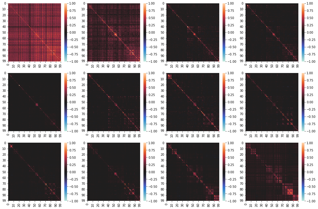
Cosine Similarity of Attention Blocks
The token cosine similarity for attention blocks at different layers ( 0, … 31 )
0-9 first digit indicates which of 10 texts is being looked at ( see above )
0-9 second digit denotes index of token vector ( 475, 479, … 511 )
The behaviour here has obvious similarities with the smaller model:
The tokens first look very similar and difficult to distinguish.
The overall similarity seems to fade in the first few layers, and similarity increases so that it is only high between inputs of similar category.
Now even the similar modules seem to fade such that none of the tokens seem particularly similar at all, even within the same text. ( small background hints seem to remain, but that are tiny compared to the size of the token )
Similarity from within the same text seems to emerge in leading up to the final layers
The similarity between categories becomes very similar again
All of the tokens begin to look very similar again, with some little cosine similarity between items in the same category..
Cosine Similarity of Decoder Blocks
The token cosine similarity for attention blocks at different layers ( 0, … 31 )
0-9 first digit indicates which of 10 texts is being looked at ( see above )
0-9 second digit denotes index of token vector ( 475, 479, … 511 )
The cosine similarity of outputs from the decoder blocks on each layer again seems to have a similar behaviour to the small model:
There is initially a very amount of similarity between all the tokens
The similarity slowly dwindles away
There slowly emerge patterns of similarity between similar-category texts
Streams of Hidden-State Dimensions
We again looked at a small number of streams of the hidden-state dimensions.
Token Embedding dimension 13 over various layers. Left: zoomed in, out: zoomed out.
The dimension 13 seems to have a very clear separation of streams for different texts, this seems to look very promising for showing some kind of modularity.
69th and 256th Token Embedding Dimensions.
Some other dimensions, such as 69 and 256 seem more typical, with the streams possibly having some correlations but they are not as clear as in dimension 13.
Conclusion: Further research seems valuable
There seems to be a sufficient amount of similarity in the activation between layers of the tokens that there could be some modular structure in the transformer. In particular, the similarity metrics seem to show similar activation patterns for tasks requiring similar knowledge and style.
However, it still seems possible that here that the similarity might come more from the specific knowledge instead of the style of the text, and in particular, there seemed to be little similarity between the different Vox articles, and it would be interesting to be able to detect such a thing.
One thing that could be considered in further research, is doing some more advanced analysis with a greater variety of inputs. One could, for example, at existing transformer interpretability research, and use tools such as Principal Component Analysis (PCA) to build a better metric than the raw Cosine Similarity, or try to visualise things with PHATE Dimension Reduction.
In addition, some of the analysis assumes a specific ontology, such as when analysing the streams of the different dimensions of the embedded vectors. There may be a better way to look at the data, such as finding directions that are not along the euclidean dimensions.
Path To Impact:
If Transformer architectures become the future path to Transformative AI, then it seems important to be able to understand them correctly. It would be useful to be able to do a neuroscience-like analysis to identify parts of the transformers that do different things ( if this is at all possible ).
One ultimate goal might be to be able to identify modules that are able to perform specific tasks, or embed the knowledge of specific simulacra. An optimal example might be to identify the “coding” part of the module, and modify the network to remove all irrelevant modules, such that one could input a text of Shakespeare, and get the model to consistently output things that look like code.
Appendix A—More Details on OPT:
In OPT-125M, Each Decoder Block has:
The Input
A Normalisation Block
An attention block with 12 attention heads
A Residual connection
Another Normalisation Block
A Dense block connecting 768 nodes to 3072 nodes to 768 nodes.
Another Residual Connection
The Output
See the original code definition, or the PyTorch summary of the decoder layers is here:
OPTDecoderLayer(
  (self_attn): OPTAttention(
    (k_proj): Linear(in_features=768, out_features=768, bias=True)
    (v_proj): Linear(in_features=768, out_features=768, bias=True)
    (q_proj): Linear(in_features=768, out_features=768, bias=True)
    (out_proj): Linear(in_features=768, out_features=768, bias=True)
  )
    (activation_fn): ReLU()
    (self_attn_layer_norm): LayerNorm((768,), eps=1e-05, elementwise_affine=True)
    (fc1): Linear(in_features=768, out_features=3072, bias=True)
    (fc2): Linear(in_features=3072, out_features=768, bias=True)
    (final_layer_norm): LayerNorm((768,), eps=1e-05, elementwise_affine=True)
)
Appendix B—Individual Attention Heads
EDIT: This section was added because I decided after reading a comment by Lucius Bushnaq that maybe I should also have included results from individual attention heads.
I also added a graph showing width of the tight-pass over time above.
The main flaws with cosine similarity are that:
It does not preserve scale well, so almost-zero and very large vectors have the same magnitude in similarity calculations.
It doesn’t show two small vectors as close to each other and far from a very large vector.
A better metric might be something like a Euclidean norm, but the norm I have been looking at while doing research for this post is a “scaled cosine similarity”. This is calculated the same as normal cosine similarity, but the vectors preserve the original ratios of length.
Here are some example graphs, calculated and labeled as before, except with “scaled cosine similarity”
Attention Block Outputs (Without Residual)
We see here that the characterisation of the behaviour is quite similar, but you can better see how the different input texts have different magnitude outputs.
Decoder Layer Output (With Residual)
These show a similar behaviour, but the sizes of the activations are better preserved
- Research agenda: Formalizing abstractions of computations by (2 Feb 2023 4:29 UTC; 93 points)
- EA & LW Forums Weekly Summary (5 − 11 Sep 22’) by (EA Forum; 12 Sep 2022 23:21 UTC; 36 points)
- Subsets and quotients in interpretability by (2 Dec 2022 23:13 UTC; 26 points)
- EA & LW Forums Weekly Summary (5 − 11 Sep 22′) by (12 Sep 2022 23:24 UTC; 24 points)
Is the idea with the cosine similarity to check whether similar prompt topics consistently end up yielding similar vectors in the embedding space across all the layers, and different topics end up in different parts of embedding space?
Because individual transformer layers are assumed to only act on specific sub-spaces of the embedding space, and write their results back into the residual stream, so if you can show that different topics end up in different sub-spaces of the stream, you effectively show that different attention heads and MLPs must be dealing with them, meaning totally different parts of the network are active for different prompts?
If that’s the idea, have you considered just logging which attention heads and MLP layers have notably high or notably low activations for different vs. similar topics instead?
This wouldn’t be an option if we were looking for modularity in general, because the network might still have different modules for dealing with different computational steps of processing the same sort of prompt.
But if your hypothesis is specifically that there are different modules in the network for dealing with different kinds of prompt topics, that seems directly testable just by checking if some sections of the network “light up” or go dark in response to different prompts. Like a human brain in an MRI reacting to visual vs. auditory data.
On first glance, this seems to me like it’d be more precise and reliable than trying to check whether different prompt topics land in different parts of the residual stream, and should also yield more research bits, because you actually get to immediately see what the modules are.
Or am I just misunderstanding what you’re trying to get at here?
Quibble: I suspect that the measure may have a lot of problems for MLPs as well. Graph theory implicitly assumes that all nodes are equivalent. If you connect two nodes to a third node with positive weights, graph theory thinks the connecti-ness from the two adds up.
But in neural networks, two different neurons can have both entirely different, or very similar features. If these features have big “parallel[1]” components with opposite sign, connecting to those neurons with positive weights can have the signals from both mostly cancel each other out[2].
Parallel in function space that is.
I think the solution to this might be to look at the network layers in a basis where all features are orthogonal.
Yeah, I would say this is the main idea I was trying to get towards.
I think I probably just look at the activations instead of the output + residual in further analysis, since it wasn’t particularly clear in the outputs of the fully-connected layer, or at least find a better metric than Cosine Similarity. Cosine Similarity probably won’t be too useful for analysis that is much deeper, but I think it was sort of useful for showing some trends.
I have also tried using a “scaled cosine similarity” metric, which shows essentially the same output, though preserves the relative length. (that is, instead of normalising each vector to 1, I rescaled each vector by the length of the largest vector, such that now the largest vector has length 1 and every other vector is smaller or equal in size).
With this metric, I think the graphs were slightly better, but the cosine similarity plots between different vectors had the behaviour of all vectors being more similar with the longest vector which I though made it more difficult to see the similarity on the graphs for small vectors, and felt like it would be more confusing to add some weird new metric. (Though now writing this, it now seems an obvious mistake that I should have just written the post with “scaled cosine similarity”, or possibly some better metric if I could find one, since it seems important here that two basically zero vectors should have a very high similarity, and this isn’t captured by either of these metrics). I might edit the post to add some extra graphs in an edited appendix, though this might also go into a separate post.
As for looking at the attention heads instead of the attention blocks, so far I haven’t seen that they are a particularly better unit for distinguishing between the different categories of text (though for this analysis so far I only looked at OPT-125M). When looking at outputs of the attention heads, and their cosine similarities, usually it seemed that the main difference was from a specific dimension being particularly bright, rather than attention heads lighting up to specific categories (when looking at the cosine similarity of the attention outputs). The magnitude of the activations also seemed pretty consistent between activation heads in the same layer (and was very small for most of the middle layers), except for the occasional high-magnitude dimension in the layers near the beginning and end.
I made some graphs that sort of show this. The indices 0-99 are the same as in the post.
Here is some results for attention head 5 from the attention block in the final decoder layer for OPT-125M:
The left image is the “scaled cosine similarity” between the (small) vectors (of size 64) put out by each attention head. The second image is the raw/unscaled values of the same output vectors, where each column represents an output vector.
Here are the same two plots, but instead for attention head 11 in the attention block of the final layer for OPT-125M:
I still think there might be some interesting things in the individual attention heads, (most likely in the key-query behaviour from what I have seen so far), but I will need to spend some more time doing analysis.
This is the analogy I have had in my head when trying to do this, but I think a my methodology has not tracked this as well as I would have preferred. In particular, I still struggle to understand how residual streams can form notions of modularity in networks.
Nice work!
Some comments on interpretation of some of the graphs:
SVD graphs: most singular value implementations are only precise to singular values of ~1e-8 times the maximum singular value. So in those graphs where the singular values fall off sharply to about 1e-7 (with maximum singular value about 1e1 or 1e2), and then flatten out, what’s actually going on is almost certainly that the later singular values are basically zero and are dominated by noise from numerical imprescision.
Also in those graphs: it looks like there is a “tight pass” from the first ~tens of singular values, which are an order of magnitude higher than the relatively-flat slope afterwards.
Cosine similarity graphs: boy, those sure do look diagonal plus low rank. I wonder what the dimension of the low rank components is, and if they correspond to anything meaningful.