TLDR: This post distills Dynamical and Bayesian Phase Transitions in a Toy Model of Superposition by Chen et al. (2023), where they study developmental stages of the Toy Model of Superposition, understanding growth and form from the perspective of Singular Learning Theory (SLT).

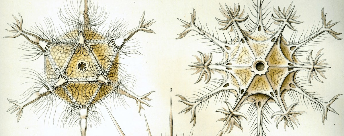
Ernst Haeckel’s *Kunstformen der Natur* (1904), plate 1: Phaeodaria

Where do the bewildering and intricate structures of Nature come from? What purpose do they serve? In his famous 1917 book “On Growth and Form” the Scottish biologist and mathematician D’Arcy Wentworth Thompson wrote the following about the geometric forms of Phaeodaria, shown above:

Great efforts have been made to attach a “biological meaning” to these elaborate structures and “to justify the hope that in time their utilitarian character will be more completely recognised”—“On Growth and Form” p. 695

Chris Olah, who pioneered mechanistic interpretability for neural networks and is somewhat of an intellectual descendant of D’Arcy Wentworth Thompson, has often cited biology as an inspiration for his work. Indeed, in many respects trained neural networks are more similar to biological organisms than to traditional computer programs. One of the most striking parallels is that, just as in biology, structure often forms over neural network training in what appear to be developmental stages.

**Developmental Stages of TMS**
First row, left: columns of the weight matrix $W$ for the function $ReLU (W^{T} W x + b)$ .
First row, right: magnitudes of columns $W_{i}$ of $W$ and associated biases $b_{i}$ .
Bottom row: losses and model complexity estimator $^λ$ over training.

In 2022, Elhage et al. introduced the Toy Model of Superposition (TMS) to study when and how models represent more features than they have dimensions, aiming to discern a method to systematically enumerate all features in a model to improve interpretability. Here, we show one case of this model: a neural network trying to reconstruct six-dimensional sparse inputs by encoding them non-linearly in two dimensions. A visualization of the encoding strategy (weights of the neural network) is shown in the top left, and it is visible that over training the network passes through three “forms” or stages of development (labelled $4^{+ + -}$ , $4^{+}$ , $5$ for reasons that will be explained below), separated by sudden transitions where the structure changes. From here on we will refer to this animation as the Developmental Stages of TMS.

What are these stages of development and what kind of process are these transitions? Can we understand why the training process passes through these particular stages in this particular order? Does this toy model reveal a path towards a better understanding of the bewildering and intricate structure of larger neural networks?

In Chen et al (2023), it is shown that the stages of development in TMS can be concretely understood from the perspective of singular learning theory. These stages (or forms) are synonymous with critical points of the loss landscape $L (w)$ , and the development between stages (growth) corresponds to phase transitions between these critical points, where the only dynamically-permissible transitions involve decreasing loss $L (w)$ and increasing model complexity $λ$ .

Let us elaborate.

On Growth and Form

We are familiar with the idea that a biological system might, over the course of its development from an embryo, take various forms that are stable and distinct. Like many familiar notions, the concept of a form is difficult to define in a careful way:

Thus according to Aristotle, the matter of a thing will consist of those elements of it which, when the thing has come into being, may be said to have become it; and the form is the arrangement or organization of those elements, as the result of which they have become the thing which they have. -- Britannica

Obviously.

For systems like neural networks whose development is governed by the process of gradient descent $˙ w = - \nabla L (w)$ for a potential $L (w)$ , a reasonable mathematical formalisation of the informal notion of a form is the concept of a critical point. A network parameter $w^{*} \in W$ is a critical point if all partial derivatives of the loss vanish, that is, $\nabla L (w^{*}) = 0$ . It’s a place where gradient descent slows down, or even stops.

Local minima and maxima in two dimensions are critical points familiar from high school calculus, as are saddles in three dimensions (with both increasing and decreasing directions nearby). We use three different words maxima, minima, saddle to distinguish these three kinds of local geometry.

**Taxonomy of critical points** $w^{*}$ of $L (w)$ **for** $w \in W \subset R^{2}$ .

For potentials $L (w)$ like the loss function of a neural network, there are many more kinds of critical points than these, each with their own particular local geometry. It is this geometry, and the configuration of these critical points relative to one another, which dominates the large scale behaviour of dynamical systems (Gilmore, in his text on Catastrophe Theory, calls this the Crowbar Principle).

To return then to the biological setting, we may identify forms with critical points and growth with flows between neighbourhoods of critical points.

In the Toy Model of Superposition, the forms are regular polygons, and we observe that growth is restricted to occur in a specific way: loss must go down, and complexity must go up. What we see in the specific $4^{+ + -} \to 4^{+} \to 5$ transition of the animation is actually a more general phenomena, at least in the setting of TMS, as the complexity of the polygon increases in each transition. This observation connects the dynamical transitions of neural network training to the Singular Learning Theory (SLT) theory of phase transitions. Let’s dive in.

The Zoo of TMS Critical Points

In the high-sparsity limit of the TMS potential $L (w)$ , it is possible to explicitly calculate and study critical points. The problem of classifying these critical points is similar in some respects to problems in the theory of tight frames, compressed sensing, and the Thomson problem. In the case of $r = 2$ feature dimensions, these critical points have a clear, interpretable meaning: they correspond to $k$ -gons.

The Setup

We consider a two-layer ReLU autoencoder with input and output dimension $c$ , with $r \leq c$ hidden dimensions in the network:

\begin{matrix} f : X \times W \to R^{c} f (x, w) = R e L U (W^{T} W x + b), \end{matrix}

where $w = (W, b) \in W$ . Here $W = [W_{1}, \dots, W_{c}]$ is a matrix of $c$ column vectors $W_{i} \in R^{r}$ , and $b \in R^{c}$ is a bias.

In the high-sparsity limit, an input sample $x \in X = [0, 1]^{c}$ from the true data-generating distribution $q (x)$ has the form $x = μ e_{i}$ , where $e_{i}$ is the $i$ th basis vector drawn uniformly from $i \sim {1, \dots, c}$ , and $μ$ is uniformly sampled from $μ \sim [0, 1]$ .

The objective of the TMS learning machine is to find an efficient method to compress the high-dimensional true input distribution $q (x)$ into a lower-dimensional representation, in other words, to approximately reconstruct any input $f (x, w) \approx x$ using less feature dimensions $r$ than input dimensions $c$ . So for any dataset of samples $D_{n} = {x_{1}, \dots, x_{n}}$ , the empirical TMS loss to minimise during training is

L_{n} (w) = \frac{1}{n} n \sum 1 = 1 ∥ x_{i} - f (x_{i}, w) ∥^{2} .

We refer to $L (w) = E [L_{n} (w)]$ as the TMS potential, for which a closed form expression is given in Lemma 3.1 of Chen et al. (2023).

TMS Critical Points are $k$ -gons

When we set the number of feature dimensions to $r = 2$ , meaning the autoencoder has $c$ weight vectors $W_{i} \in R^{2}$ in the plane to perform its compression, the most interesting low-loss critical points^[1] are regular polygons — triangles, squares, pentagons and the like. Each critical point $w^{*} = (W^{*}, b^{*})$ is characterised by three quantities:

$k$ : the number of vertices $k \leq c$ in the regular polygon formed by the convex hull of the columns of the $W^{*}$ .
$σ$ : the number of positive values in the bias vector $b^{*}$ .
$ϕ$ : the number of large negative values in $b^{*}$ .

We denote each critical point as a $k^{σ +, ϕ -}$ -gon, which we will call $k$ -gon for short.^[2] These are the fundamental forms of the Toy Model of Superposition.

**Three** $k$ **-gons**: a $4^{+ + -}$ -gon, a $4^{+}$ -gon, and a $5$ -gon, all seen in the **Developmental Stages of TMS** animation. For each $k$ -gon, the left diagram depicts the vectors $W_{i} \in R^{2}$ , and the right diagram depicts the magnitudes $∥ W_{i} ∥$ (black), and $| b_{i} |$ (red if $b_{i} < 0$ , green if $b_{i} > 0$ ) for each $i = 1, \dots, c$ .

In the $r = 2, c = 6$ case, we empirically catalogued and theoretically proved the existence of 18 low-loss critical points.^[3] Since we have a closed form expression for the TMS potential $L (w)$ , we can easily plug in each identified critical point to find its loss and create a diagram akin to the energy-levels of different states in physics.

**Energy Levels of** $k$ **-gons:** The loss $L (w)$ (aka “energy”) evaluated at each of the 18 catalogued $k$ -gons for $r = 2, c = 6$ , accompanied by its corresponding $k^{σ +, ϕ -}$ -gon configuration on the right.

SGD Plateaus at $k$ -gons

The Developmental Stages of TMS animation shows SGD settling at three different plateaus through training, which we visually saw corresponded to different “forms” of the parameter $w = (W, b)$ . These forms are different $k$ -gon critical points, each with their own loss plateau.

This is not a one-off.

**SGD Plateaus:** Energy levels $L (w (t))$ of SGD trajectories at time $t$ . The trajectory always settles on a loss plateau corresponding to a different $k$ -gon.

No matter where SGD is initialised, it always plateaus on a known $k$ -gon critical point. Sometimes it even transitions through multiple plateaus, like we see in the animation.

So, in TMS, SGD training trajectories can be thought of as a developmental journey through different $k$ -gon forms. The rapid drops in loss from plateau to plateau signify instances of actual growth. For example, the model literally develops a new limb when it transitions from a $4^{+}$ -gon to a $5$ -gon.

Opposing Staircases: Loss ↓, Complexity ↑

Let’s take a closer look at the green line in the Developmental Stages of TMS animation, which we have claimed is measuring the “local complexity” $^λ (t)$ of the model at time $t$ . (Why we care about the local complexity $^λ$ will be explained below).

Notice how as loss goes down over training, the local complexity goes up, as if they’re opposing staircases.

**Opposing staircases**: As SGD moves down through different loss plateaus, it simultaneously moves up through different complexity plateaus. The green line denotes lambdahat $^λ (t)$ estimates over time. The three red dots on the loss curve denote the three $k$ -gon snapshots seen above.

In fact, if we look back at the colourful SGD Plateaus plot above, there seems to be an inverse relationship between the energy $L (w_{α}^{*})$ of a critical point $w_{α}^{*}$ and its estimated complexity ${^λ}_{α}$ , suggesting a more general phenomena than just the $4^{+ + -} \to 4^{+} \to 5$ transition we see here.

One can plot $({^λ}_{α}, L (w_{α}^{*}))$ for different $k$ -gon critical points $w_{α}^{*}$ , and then connect the pairs between which there were observed phase transitions in SGD. In doing this we repeatedly observe this same pattern: structure seems to form in particular ways, consistently decreasing loss while increasing complexity. Some transitions are dynamically permissible, and others aren’t.

This single plot of loss against complexity captures the growth and form of TMS.

**Loss and complexity of** $k$ **-gons:** The pairs $({^λ}_{α}, L (w_{α}^{*}))$ for 14 of our 18 catalogued $k$ -gon critical points. Red lines connect the critical points between which we observe dynamical transitions. There appears to be a logic to the formation of structure—not all transitions are permissible from SGD’s point of view. In all cases, a decrease in loss is accompanied by an increase in complexity.

What explains these highly restricted developmental trajectories? Training often skips past critical points with intermediary energy levels, so it can’t simply be a case of moving further and further down the loss landscape. Something else is going on.

Singular learning theory (SLT) can shed some light.

TMS meets SLT

Bayesian Phases are also Critical Points

Phases Minimise the Free Energy

Those already familiar with the general story we have been telling will recognise that there is a better name for these “forms” that we observe throughout TMS training. They are phases. Moreover, the sharp drops between plateaus are indicative of growth in structure, and these are phase transitions.

Plateaus in loss are sometimes referred to informally as phases in the machine learning literature. To get to the heart of this, we turn to the Bayesian perspective on learning. Here the posterior $p (w | D_{n}) \propto e^{- n L_{n} (w)} φ (w)$ (for some prior $φ (w)$ on parameter space $W \subset R^{d}$ ) is the central object, containing all information about our system for any sample size $n$ .

In statistical physics and Bayesian learning theory a phase is some region $W_{α}$ of state/parameter space $W$ that has concentrated posterior mass — in other words, a configuration of the system that the posterior deems likely to occur. This posterior mass is measured (for tractability reasons) using the free energy $F_{n} (W_{α})$ ^[4]. The Bayesian model selection process is then guided by the principle of free energy minimisation (equivalently, posterior mass maximisation).

**Phases of a Bayesian Posterior:** A posterior defined by $p (w | D_{n}) = e^{- n L (w)}$ where $L (w) = (w_{1} - 1)^{2} (w_{1}^{2} + w_{2}^{2} + 1 / 4)^{4}$ , seen here for $n = 10$ and $n = 100$ .
There are two natural phases with concentrated posterior mass for this posterior: a ball $W_{1}$ centred at $w = (0, 0)$ , and a region $W_{2}$ around the line ${w : w_{1} = 1}$ .
These two phases have different geometric characters, i.e. differing loss and complexity.

So are Bayesian phases also related to critical points of $L (w)$ ? They sure are.

Geometric Signatures of Bayesian Phases

Let $W_{α}$ be a region of parameter space $W \subset R^{d}$ that contains a critical point $w_{α}^{*}$ , where $w_{α}^{*}$ locally minimises the loss $L (w) = E [L_{n} (w)]$ in $W_{α}$ . Then as the number of samples $n$ tends to infinity, Watanabe’s free energy formula tells us that the local free energy of $W_{α}$ is asymptotically given by

F_{n} (W_{α}) \approx n L_{n} (w_{α}^{*}) + λ_{α} log n + c_{α} as n \to \infty .

Here $n L_{n} (w_{α}^{*})$ is the loss (aka potential energy), $λ_{α} \in Q_{> 0}$ is the local learning coefficient (aka model complexity, aka the RLCT), and $c_{α}$ includes a term of order $log log n$ and a constant order term which incorporates information such as the prior-volume (or equivalently in this setting, the weight-norm $∥ w ∥^{2}$ ). ^[5]

This formula tells us that the posterior concentrates on neighbourhoods of critical points $W_{α}$ , which we will now genuinely call phases in good conscience. Remember, singular models like neural networks induce loss landscapes $L (w)$ that have a diverse set of critical points with differing tradeoffs between loss and complexity, unlike regular models where complexity $λ$ is constant across parameter space, $λ = \frac{d}{2}$ .

That these local geometries vary across parameter space is what gives singular models their rich phase structure. This is exactly what we saw with the diverse catalogue of TMS $k$ -gon phases, each having different loss-complexity tradeoffs $({^λ}_{α}, L (w_{α}^{*}))$ .

What does SLT say about phase transitions, though?

Bayesian Phase Transitions

Internal Model Selection

The different tradeoffs between loss and complexity across phases result in what is effectively internal model selection. The posterior prefers high-loss-low-complexity models $W_{α}$ in the face of insufficient evidence (low $n$ ) — a kind of Occam’s Razor — but, as you increase your evidence with more training samples $n$ , the posterior becomes more certain that low-loss-high-complexity models $W_{β}$ are better.

This process forms the basis of Bayesian phase transitions, which occur when there is a sudden change in which region of parameter space has the dominant posterior mass (equivalently, lower free energy).

Suppose we carve up (or more precisely, coarse grain) our parameter space $W \subset R^{d}$ into a finite set of disjoint phases ${W_{α}}_{α}$ covering $W$ . (Precisely how you coarse grain parameter space to perform maximally interesting inference is a non-trivial process—in TMS this is natural, in other settings it may not be).

By the log-sum-exp-approximation, the global free energy $F_{n}$ defined by $e^{- F_{n}} = \sum_{α} e^{- F_{n} (W_{α})}$ is approximately

\begin{matrix} F_{n} & = - log \sum α e^{- F_{n} (W_{α})} \approx min α F_{n} (W_{α}) \approx min α [n L_{n} (w_{α}^{*}) + λ_{α} log n + c_{α}], \end{matrix}

meaning that it is dominated by the phase $W_{α}$ with the lowest free energy for a given $n$ value, while the rest are exponentially suppressed. This is the sense in which the posterior “chooses” the phase $W_{α}$ at a given $n$ .

Phase Transitions from High-Loss-Low-Complexity to Low-Loss-High-Complexity

So when does the dominant phase change from the point of view of the free energy? In the simplest case, say we had two phases $α$ and $β$ , defined by neighbourhoods $W_{α}$ and $W_{β}$ centred at critical points $w_{α}^{*}$ and $w_{β}^{*}$ respectively. Let’s suppose that $β$ has better loss but higher complexity, so

Δ L = L_{n} (w_{β}^{*}) - L_{n} (w_{α}^{*}) < 0 and Δ λ = λ_{β} - λ_{α} > 0,

(and suppose that $c_{α} - c_{β} = 0$ for ease). Then as $n$ increases, a Bayesian phase transition from $α \to β$ will occur at $n \approx n_{crit}$ when the ordering of their free energies flips. Solving $F_{n} (W_{α}) = F_{n} (W_{β})$ shows that $n_{crit}$ is the unique solution to ^[6]

n Δ L + Δ λ log n = 0 .

We say there is a Bayesian phase transition of Type A at $n = n_{c r}$ .

Are visions of opposing staircases flashing before your eyes?

**Bayesian phase transitions:**
Plotting $F_{n} (W_{α}) = n L_{n} (w_{α}^{*}) + λ_{α} log n + c_{α}$ versus $n$ for different phases $α$ , a Bayesian phase transition occurs at $n_{crit}$ when there is a new phase with minimum free energy.

Perhaps Dynamical Transitions have Bayesian Antecedents

A Bayesian transition occurs as we increase sample size $n$ , whereas dynamical transitions occur in SGD time $t$ . We know that both are governed by the critical points $L (w)$ . But is there a deeper connection going on?

**Transitions in critical points across** $W$ . Here, black lines represent minima (singularities) of $L (w)$ .
**Bayesian (left):** The theory of phase transitions in SLT is grounded in a Bayesian formalism. Like thermodynamics, there are essentially no dynamics: transitions involve discrete changes in your probability density over state space as you change some control variable.
**Dynamical (right):** It remains unclear what this theory has to say about *dynamical phase transitions* in SGD timesteps.

The Toy Model of Superposition suggests there is. In both settings, transitions occur from high-loss-low-complexity $k$ -gons to low-loss-high-complexity $k$ -gons, suggesting that any dynamical system has a Bayesian phase transition “standing behind it”, which we will call a Bayesian antecedent.

This observation leads us to put forward the following hypothesis:

Bayesian Antecedent Hypothesis (BAH): The dynamical transitions $α \to β$ encountered in neural network training have Bayesian antecedents.

When operationalised in the TMS setting for a transition $α \to β$ in time, and assuming that only Type A transitions occur, the BAH implies:

When we see a drop in loss $L_{β} < L_{α}$ we should see an accompanying rise in learning coefficient $λ_{β} > λ_{α}$ .
If there are multiple transitions, the gradient $\frac{Δ L}{Δ λ}$ should increase (negative slope become shallower) for consecutive transitions.

This was not falsified in the TMS experiments.

Do Bayesian Phase Transitions even exist? Yes!

“Wait a second, didn’t you say the free energy formula is an asymptotic approximation? Why should I believe it for finite $n$ , let alone moderately sized $n$ ? Do these Bayesian phase transitions even exist, empirically?”

Yes, yes they do.

Returning to our catalogue of $k$ -gon critical points, we are actually able to theoretically calculate the learning coefficient of the 5- and 6-gons^[7]:

Phase $α$	Local Learning Coefficient $λ_{α}$	Loss $L_{n} (w_{α}^{*})$	Constant $c_{α}$
5-gon	7	0.06874	$>$ 3.62417
$5^{+}$ -gon	8.5	0.06180	3.62764
6-gon	8.5	0.04819	6.37767

Running the numbers, the free energy formula theoretically predicts that there will be a phase transition at $n_{crit} = 601$ , which we can verify empirically by using MCMC to sample from the TMS posterior distribution at a range of dataset sizes $n$ .

Crucially, because we know the critical points in TMS are $k$ -gons, we are able to very naturally coarse-grain parameter space into phases ${W_{α}}_{α}$ , thereby assigning any posterior sample $w = (W, b)$ into a phase. This feature of TMS allows us to calculate the relative frequency of each phase for different $n$ , i.e. the probability mass

P (w \in W_{α} ∣ D_{n}) = \frac{e^{- F_{n} (W_{α})}}{\sum_{β} e^{- F_{n} (W_{β})}}

for each phase $W_{α}$ . Plotting these relative frequencies over a range of $n$ gives us phase occupancy curves, allowing us to compare the theoretical occupancy curve (determined by the theoretical $L_{n} (w_{α}^{*}), λ_{α}, c_{α}$ ) and the empirically derived version from MCMC experiments.

**A real Bayesian phase transition:** Theoretical (left) vs empirical (right) occupancy curves as $n$ varies, showing a Bayesian phase transition from the $5$ -gon to the $6$ -gon at $n_{crit} \approx 600$ .

The most salient feature of the curves is the Bayesian phase transition from a $5 -gon \to 6 -gon$ which happens at the crossover around $n_{crit} \approx 600$ , seen in both the theoretical and empirical curves (and occurring at remarkably similar values of $n$ ). Since the 6-gon is the global minimum of the TMS potential $L (w)$ for $r = 2, c = 6$ , it is not surprising to see that it is the eventual dominant phase for sufficiently large $n$ . But just as SLT predicts, since the 5-gon has lower complexity, it can be the dominant phase for some range of $n$ , which we see here for $n \in [100, 600]$ .

It’s worth noting that for low $n$ , a lot of this analysis does start to break down. This is primarily because the lower order terms of the asymptotic free energy formula become increasingly more important, and classifying each sample into a phase becomes less precise due to a more diffuse posterior. ^[8]

To guard against some of these issues, one can manually inspected MCMC samples using a 2D t-SNE projection to verify that the phase classifications do cluster together appropriately.

**t-SNE visualisation of MCMC samples** **for** $n = 300, 500, 700, 1000$ .
Observe that the change in cluster size of the 5 and 6-gon and the gradual suppression of other phases.
See interactive version here: http://project-tms.s3-website-ap-southeast-2.amazonaws.com/

Updates and where to now?

The work presented here represents the first step toward not just verifying some of the key tenets of the developmental interpretability agenda but also advancing toward a science of deep learning through the thermodynamic lens of singular learning theory.

Some updates we took away from working on this:

SLT works, folks. This is the first empirical verification of the predictive power of the SLT theory of phase transitions outside of some synthetic examples. That Bayesian phase transitions are a real phenomena at moderately sized $n$ (our MCMC experiments ranged from $n \in [100, 1200]$ ) is a substantial piece of evidence that SLT is relevant to “real systems”.
Dynamical phase transitions are related to Bayesian ones: We know that both kinds of transitions are governed by the critical points of $L (w)$ , but aside from this, there is no a-priori relation between the two. With TMS, we now have a real (albeit toy) system that exhibits the behaviour we hypothesised in the devinterp agenda relating dynamical phase transitions to those predicted by singular learning theory.
Lambda-hat works. We have a measure of model complexity and it correctly describes phase transitions. This was a major question mark previously.

It’s worth pausing here for a moment to consider the parts of this work that are specific to TMS (“mechanistic” claims, specific to the problem at hand) and those that we expect to hold more broadly (“thermodynamic” claims, true across general learning machines).

Here are some examples:

Mechanistic claims	Thermodynamical claims
$k^{σ + ϕ -}$ -gons are critical points.	The posterior concentrates near critical points.
SGD training proceeds by forming increasingly complex polygons.	SGD and Bayesian learning proceed via phase transitions.
A 4-gon can transition to 5-gon during SGD training.	Bayesian and dynamical transitions decrease the free energy.
Higher energy $k^{σ + ϕ -}$ -gon phases have mostly lower complexity.	There are “phase structures” that relate energy and complexity of phases.

Obviously we don’t expect to see $k$ -gons as critical points in general networks. These structures/forms/phases will manifest in many different ways. But we do expect them to form in phase transitions as a universal phenomena.

Some of the guiding questions from here include:

Can we develop and refine tools such as lambda-hat $^λ$ that allow us to detect phase transitions, even without knowing the phases of the system?
Do dynamical phase transitions in other systems also have Bayesian antecedents? Just how far does the BAH apply beyond TMS?
Can we use further insights of SLT to extrapolate a deeper understanding of structure formation not just in toy cases, but in large language and vision models?

We believe that understanding the growth and form of neural networks is fundamental to a science of deep learning, and that this understanding will come from a combination of deep mathematics and careful study of many particular systems, like TMS. In this we take inspiration from D’Arcy Wentworth Thompson, who had a passion not only for mathematics, but for collating many beautiful examples of organism development from across the natural world.

Thanks to @Daniel Murfet , @Jesse Hoogland and @Alexander Gietelink Oldenziel for reviewing earlier drafts of this distillation!

^
Here we are slightly abusing the term “critical point”—in general, we are actually referring to critical submanifolds. In the case of the TMS potential, there are two generic symmetries that mean the different “critical points” are actually critical submanifolds:
Permutation symmetry, where, like any other feedforward ReLU neural network we can permute hidden nodes (i.e. simultaneously permute weight columns and bias entries) and still yield the same function, and;
Rotation symmetry, (or more precisely, $O (r)$ -invariance, where $O (2)$ is rotation in the plane), since for any orthogonal matrix $O \in R^{r \times r}$ we have
$f (x, (O W, b)) = R e L U (W^{T} O^{T} O W x + b) = R e L U (W^{T} W x + b) = f (x, (W, b)) .$
These generic symmetries mean that singular learning theory is an essential tool to fully understand the TMS system.
^
There are some proven constraints on what combinations of $(k, σ, ϕ)$ are possible—for more details, see Appendix A of Chen et al. (2023).
^
While we have not proven that these are all of the possible critical points (and indeed, there are likely many more high-loss critical points that SGD never cares about), we are confident that we found all of the important ones.
^
For a given region of parameter space $W_{α} \subset W$ the free energy is
$F_{n} (W_{α}) = - log (\int_{W_{α}} e^{- n L_{n} (w)} φ (w) d w),$
thus measuring the posterior concentration of $W_{α}$ .
^
To be clear, this is the free energy to leading order. It is an active problem to determine lower order terms of the free energy, investigating which other geometric quantities are important for model selection.
^
The precision of this $n_{crit}$ value is not to be taken too literally—it is, after all, based on an asymptotic approximation. Interpreting such asymptotics require great care for any finite- $n$ system (which is all we ever care about in real systems).
^
In fact, we actually have a reasonably good idea of learning coefficients for various $4^{σ +, ϕ -}$ -gons too, however these remain unpublished due to some technical non-analyticity complications.
^
Such analysis also depends on the coarse graining of the phases, and while we are quite sure we have located all low-energy critical points, it is still possible that the presence of other unaccounted for phases could introduce inaccuracies in these occupancy curves.

Growth and Form in a Toy Model of Superposition