DSLT 3. Neural Networks are Singular

[Liam Carroll]

TLDR; This is the third main post of Distilling Singular Learning Theory which is introduced in DSLT0. I explain that neural networks are singular models because of the symmetries in parameter space that produce the same function, and introduce a toy two layer ReLU neural network setup where these symmetries can be perfectly classified. I provide motivating examples of each kind of symmetry, with particular emphasis on the non-generic node-degeneracy and orientation-reversing symmetries that give rise to interesting phases to be studied in DSLT4.

As we discussed in DSLT2, singular models have the capacity to generalise well because the effective dimension of a singular model, as measured by the RLCT, can be less than half the dimension of parameter space. With this in mind, it should be no surprise that neural networks are indeed singular models, but up until this point we have not exactly explained what feature they possess that makes them singular. In this post, we will explain that in essence:

Neural networks are singular because there are often ways to vary their parameters without changing the function they compute.

In the case where the model and truth are both defined by similar neural network architectures, this fact means that the set of true parameters $W_0$ is non-trivial (i.e. bigger than the regular case where it is a single point), and often possesses many symmetries. This directly implies that neural networks are singular models.

The primary purpose of this post is to show with examples why neural networks are singular, and classify the set of true parameters $W_0$ in the case where the model and truth are simple two layer feedforward ReLU networks. In doing so, we will lay the groundwork for understanding the phases present in the setup so that we can then study relevant phase transitions in DSLT4. Feel free to jump ahead to the slightly more exciting DSLT4 Phase Transitions in Neural Networks and refer back to this post as needed.

Outline of Classification

To understand the different regions that minimise the free energy (and thus, as we’ll see in DSLT4, the phases), one needs to first understand the singularities in the set of optimal parameters of $K\left(w\right)$.

In the realisable regression case with a model neural network $f(x,w)$ and true neural network defined by $f_0\left(x\right)=f(x,w^{\left(0\right)})$ for some $w^{\left(0\right)}\in W$, the set of true parameters has the form ^[1]

$$W_0=\{w\in W|f(x,w)=f_0(x\left)\right\}.$$

Thus, classifying the true parameters is a matter of establishing which parameters $w\in W$ yield functional equivalence between the model and the truth $f(x,w)=f_0\left(x\right)$. The property of being singular is specific to a model class $f(x,w)$, regardless of the underlying truth. But, classifying $W_0$ in the realisable case is a convenient way of studying what functionally equivalent symmetries exist for a particular model class.

Neural networks have been shown to satisfy a number of different symmetries of functional equivalence across a range of activation functions and architectures, which we will elaborate on throughout the post. Unsurprisingly, the nonlinearity of the activation function plays a central role in governing these symmetries. In general, then, deep neural networks are highly singular.

In this post we are going to explore a full characterisation of the symmetries of $W_0$ when the model is a two layer feedforward ReLU neural networks with $d$ hidden nodes, and the truth is the same architecture but with $m\le d$ nodes. Though you would never use such a basic model in real deep learning, the simplicity of this class of network allows us to study $W_0$ with full precision. We will see that:

• If the model and truth have the same number of nodes, $m=d$: There are three forms of symmetry of $W_0$:

  • Scaling symmetry of the incoming and outgoing weights to any node.

  • Permutation symmetry of the hidden nodes in a layer.

  • Orientation reversing symmetry of the weights, only when some subset of weights sum to zero (i.e. “annihilate” one another).

• If the model has more nodes than the truth, $m<d$: Without loss of generality, the first $m$ nodes of the model must have the same symmetries as in the first case. Then each excess node $i\in \{m+1,\dots ,d\}$ is either

  • Degenerate, meaning its total weight (gradient) is 0 (thus the node is always constant).

  • Or it has the same activation boundary as another already in the model such that the weights sum to the total gradient in a region ^[2].

In [Carroll, Chapter 4], I give rigorous proofs that in both cases, $W_0$ is classified by these symmetries, and these symmetries alone. The purpose of this post is not to repeat these proofs, but to provide the intuition for each of these symmetries. I have included a sketch of the full proof in the appendix of this post if you are more mathematically inclined.

Two layer Feedforward ReLU Neural Networks

Literature abounds on what neural networks are, so I will merely give the definition of the class we are going to study here and some related terminology for the discussion.

Defining the Networks and Terminology

Let $W\subseteq R^{4d+1}$ be a compact parameter space. We will let $\left[d\right]=\{1,\dots ,d\}$ denote the set of hidden nodes in the first layer of our network, and $⟨w_i,x⟩$ denote the standard dot product between two vectors. Also recall that

$$ReLU\left(x\right)=\{\begin{array}{cc}x& \text{if}x\ge 0\\ 0& \text{if}x<0\end{array}.$$

We let $f:R^2\times W\to R^1$ denote a two layer feedforward ReLU neural network with two inputs $x_1,x_2$ and one output $y$, defined by a parameter $w\in W$. The function is given by

$$f(x,w)=c+\sum _{i=1}^d{q}_{i}ReLU(⟨w_i,x⟩+b_i)$$

where for each $i\in \left[d\right]$:

• the first layer weights are $w_i\in R^2$ and the biases are $b_i\in R$

• the second layer weights are $q_i\in R$ and the bias is $c\in R$.

These functions are simply piecewise affine functions (i.e. piecewise hyperplanes), and as such they have (relatively) easy topology to study. Before we give an example, we will briefly mention some key terminology.

Let $f_w\left(x\right)=f(x,w)$ be defined by a fixed $w\in W$. We say a particular node $i\in \left[d\right]$ is degenerate in $f_w$ if either of the weights are zero, so $w_i=0$ or $q_i=0$. ^[3]

We say a non-degenerate node $i$ is activated in some linear domain ^[4] $U\subseteq R^2$ when the ReLU is non-zero for all $x\in U$ , that is,

$$⟨w_i,x⟩+b_i=w_{i,1}{x}_1+w_{i,2}{x}_2+b_i>0.$$

The activation boundary associated to node $i$ is thus the line

$$H_i=\{x\in R^2|⟨w_i,x⟩+b_i=0\}.$$

One of the key accounting tools in the symmetry classification is identifying the foldsets of $f_w$ (in the terminology of [PL19]), which are the regions where $f_w$ is non-differentiable in $x$, and noticing that these equate to the union of non-degenerate activation boundaries $H_i$. Two functionally equivalent networks must then have the same foldsets since they define the same function, allowing us to compare the lines defined by $H_i$.

Example—Feedforward ReLU Neural Networks are Piecewise Hyperplanes

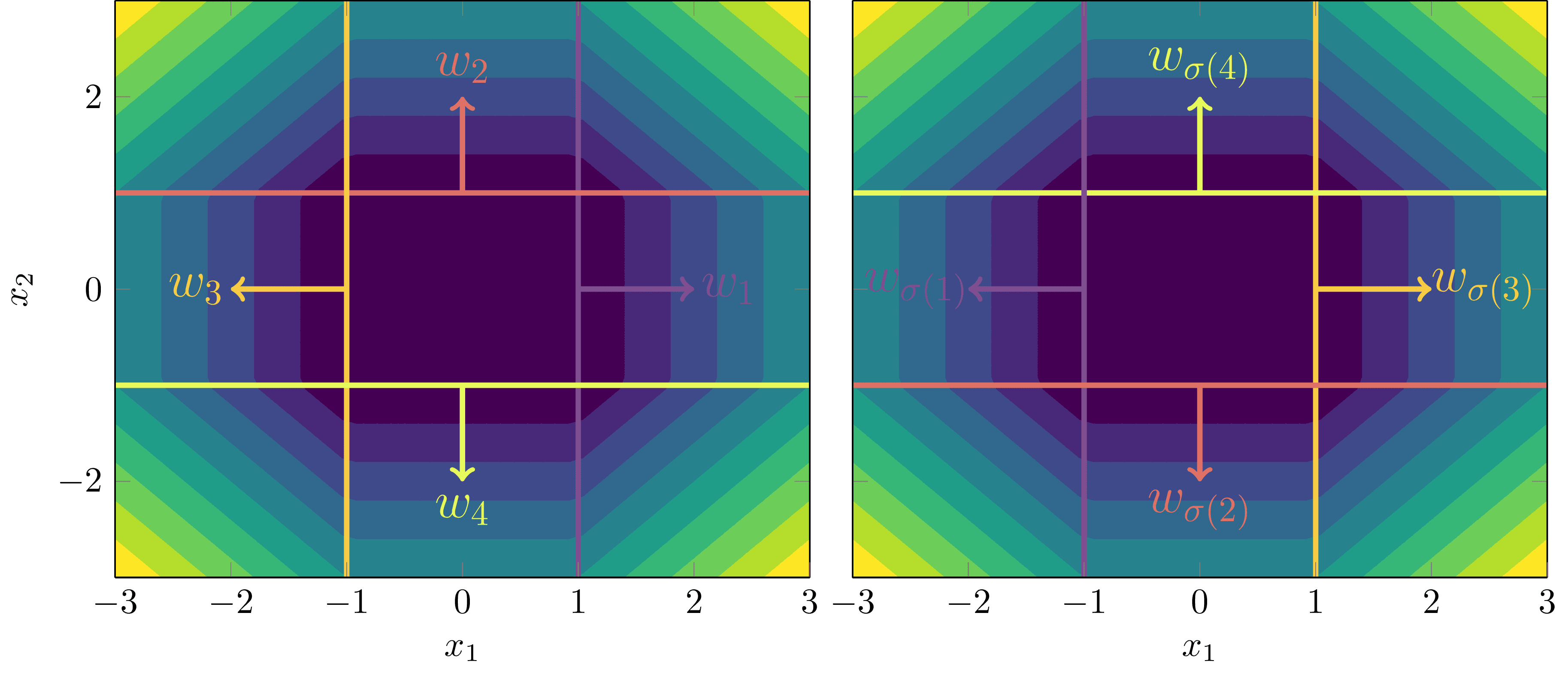
Example 3.1: Consider the following two layer feedforward ReLU neural network:

$$\begin{array}{cc}{f}_w\left(x\right)& =ReLU(x_1-1)+ReLU(x_2-1)\\ & +ReLU(-x_1-1)+ReLU(-x_2-1).\end{array}$$

defined by biases $b_i=-1$ and $c=0$, second layer weights $q_i=1$, and first layer weights

$$w_1=\left(\begin{array}{c}1\\ 0\end{array}\right),w_2=\left(\begin{array}{c}0\\ 1\end{array}\right),w_3=\left(\begin{array}{c}-1\\ 0\end{array}\right),w_4=\left(\begin{array}{c}0\\ -1\end{array}\right).$$

Its graphical structure and activation boundaries in the $(x_1,x_2)$ plane can be seen below:

The data of $f_w\left(x\right)$ above.

Conceptually, it’s helpful to notice that when anchored on its corresponding activation boundary, each weight vector $w_i$ “points” into its region of activation.

The Symmetries of Two Layer Feedforward ReLU Neural Networks

In this section I am going to provide some motivating examples of each kind of symmetry exhibited in two layer feedforward ReLU neural networks. To prove that this is the full set of symmetries in generality requires a bit more work, which we relegate to the appendix.

Scaling Inner and Outer Weights of a Node

The scaling symmetry of ReLU networks offers us our first window into why these models are singular. The key property is to notice that for any $\alpha >0$, the ReLU satisfies a scale invariance ^[5]

$$\frac{1}{\alpha }ReLU\left(\alpha x\right)=ReLU\left(x\right).$$

Say we had the simplest model possible with just one node:

$$f(x,w)=q_{1}ReLU(⟨w_1,x⟩+b_1)+c.$$

Then we could define an alternative parameter $w^{\prime }$ with

$$q_1^{\prime }=\frac{q_1}{\alpha },w_1^{\prime }=\alpha w_1,b_1^{\prime }=\alpha b_1,c^{\prime }=c,$$

which gives functional equivalence because,

$$\begin{array}{cc}f(x,w^{\prime })& =q_1^{\prime }ReLU(⟨w_1^{\prime },x⟩+b_1^{\prime })+c^{\prime }\\ & =\frac{q_1}{\alpha }ReLU(⟨\alpha w_1,x⟩+\alpha b_1)+c\\ & =\frac{q_1}{\alpha }ReLU\left(\alpha \right(⟨w_1,x⟩+b_1\left)\right)+c\\ & =q_{1}ReLU(⟨w_1,x⟩+b_1)+c\\ & =f(x,w).\end{array}$$

For a model with $d$ hidden nodes, the same scaling symmetry applies to each individual node $i\in \left[d\right]$ with a set of scaling factors ${\alpha }_i>0$.

The fact that we can define such a $w^{\prime }$ for any set of positive scalars means that the Fisher information matrix of these models is degenerate at all points $w\in W$. We prove this in generality in Appendix 1, but I’ll spell it out explicitly for a simple example here.

Example—Scaling Symmetry Induces a Degenerate Fisher Information Matrix

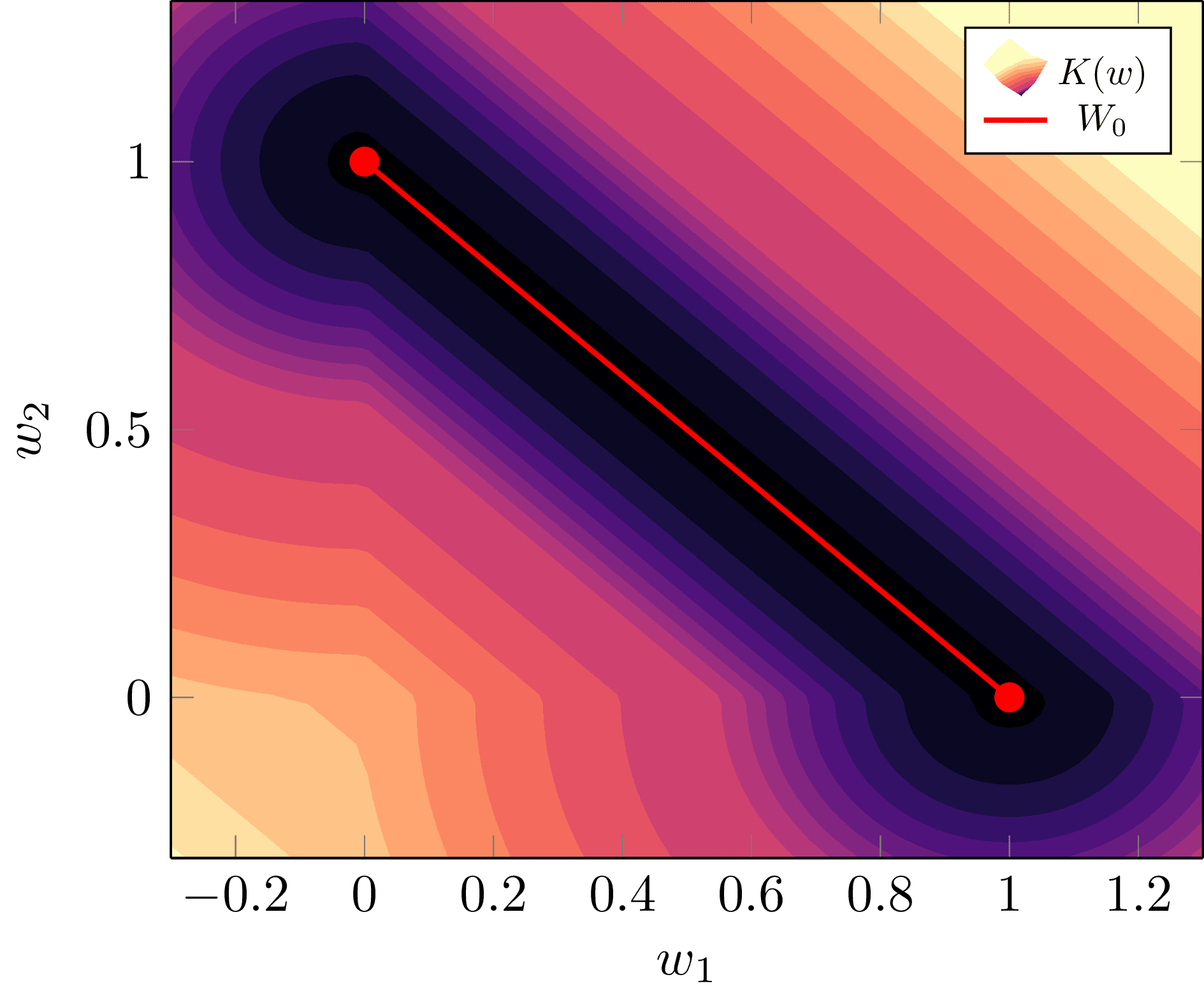
Example 3.2: It is worth taking a moment to recognise how this scaling symmetry affects the geometry of the loss landscape $K\left(w\right)$. The mental model to have here is that it results in valleys in $K\left(w\right)$, where the set of true parameters $W_0$ is like a river on the valley floor. To see this, say we defined a model with parameter $w=(w,q)$ and truth as:

$$f(x,w)=qReLU\left(wx\right),f_0\left(x\right)={\theta }_{0}ReLU\left(x\right),$$

where ${\theta }_0>0$ is some fixed constant. If $q\left(x\right)$ is uniform on $[-\sqrt{3},\sqrt{3}]$ then it is easy to calculate that when $w,q\ge 0$ we have

$$K\left(w\right)={(wq-{\theta }_0)}^2,\text{so}{W}_0=\left\{\right(w,q)|wq={\theta }_0\}.$$

We can depict this valley and its effect on the posterior for ${\theta }_0=\frac{1}{5}$:

Setting ${\theta }_0=\frac{1}{5}$, we see that $K\left(w\right)$ is a valley due to the scaling symmetry (left), thus there is no unique maximum a posterior (right). Remember that, up to a scaling factor, $e^{-n{K}_n\left(w\right)}$ is the posterior when the prior $\phi \left(w\right)$ is uniform, and $e^{-n{K}_n\left(w\right)}\approx e^{-nK\left(w\right)}$ for large $n$ since $E\left[K_n\right(w\left)\right]=K\left(w\right)$.

Looking at this $K\left(w\right)$, it’s easy to intuit that the Fisher information matrix $I\left(w\right)$ is degenerate for all $w$. But, for clarity, let me spell this out for the true parameters in the case where ${\theta }_0=1$, so $K\left(w\right)=(wq-1{)}^2$.

Remember that at true parameters the Fisher information matrix is just the Hessian, which in this case has the form

$$J\left(w\right)=\left(\begin{array}{cc}2q^2& 4wq-2\\ 4wq-2& 2w^2\end{array}\right).$$

In particular, let $w^{\left(0\right)}\in W_0$ be a fixed true parameter parameterised by a fixed $\alpha >0$, so $w^{\left(0\right)}=(\alpha ,\frac{1}{\alpha })$. Then the Fisher information matrix has the form

$$I\left(w^{\left(0\right)}\right)=\left(\begin{array}{cc}\frac{2}{{\alpha }^2}& 2\\ 2& 2{\alpha }^2\end{array}\right).$$

Setting $I_1\left(w^{\left(0\right)}\right)$ and $I_2\left(w^{\left(0\right)}\right)$ to be the rows of the matrix, there is clearly a linear dependence relation

$$-{\alpha }^2{I}_1\left(w^{\left(0\right)}\right)+I_2\left(w^{\left(0\right)}\right)=0$$

and since $\alpha$ is arbitrary, this shows that all true parameters have degenerate Fisher information matrices and are thus singular.

Permutation of Nodes

This one is easy to see. If we have a model with $d=2$ nodes,

$$f(x,w)=q_{1}ReLU(⟨w_1,x⟩+b_1)+q_{2}ReLU(⟨w_2,x⟩+b_2)+c,$$

and we define a new model $f(x,w^{\prime })$ where $w^{\prime }$ is a permutation of the nodes in $f(x,w)$,

$$(w_1^{\prime },b_1^{\prime },q_1^{\prime })=(w_2,b_2,q_2),(w_2^{\prime },b_2^{\prime },q_2^{\prime })=(w_1,b_1,q_1),\text{and}{c}^{\prime }=c,$$

then

$$\begin{array}{cc}f(x,w^{\prime })& =q_1^{\prime }ReLU(⟨w_1^{\prime },x⟩+b_1^{\prime })+q_2^{\prime }ReLU(⟨w_2^{\prime },x⟩+b_2^{\prime })+c^{\prime }\\ & =q_{2}ReLU(⟨w_2,x⟩+b_2)+q_{1}ReLU(⟨w_1,x⟩+b_1)+c\\ & =f(x,w).\end{array}$$

This easily generalises to $d$ hidden nodes by taking any permutation $\sigma \in S_d$ in the permutation group $S_d$ and letting each node $i^{\prime }$ of $f(x,w^{\prime })$ satisfy $i^{\prime }=\sigma \left(i\right)$, so

$$\begin{array}{cc}f(x,w)& =c+\sum _{i=1}^d{q}_{i}ReLU(⟨w_i,x⟩+b_i)\\ & =c+\sum _{i=1}^d{q}_{\sigma \left(i\right)}ReLU(⟨w_{\sigma \left(i\right)},x⟩+b_{\sigma \left(i\right)})=f(x,w^{\prime }).\end{array}$$

Permuting nodes induces functional equivalence, here depicted for $\sigma =(1,3)(2,4)$.

Orientation Reversal

This one is a bit trickier to observe as the symmetry depends on a very specific condition of weight annihilation. Let’s look at a simple example first.

Motivating Example

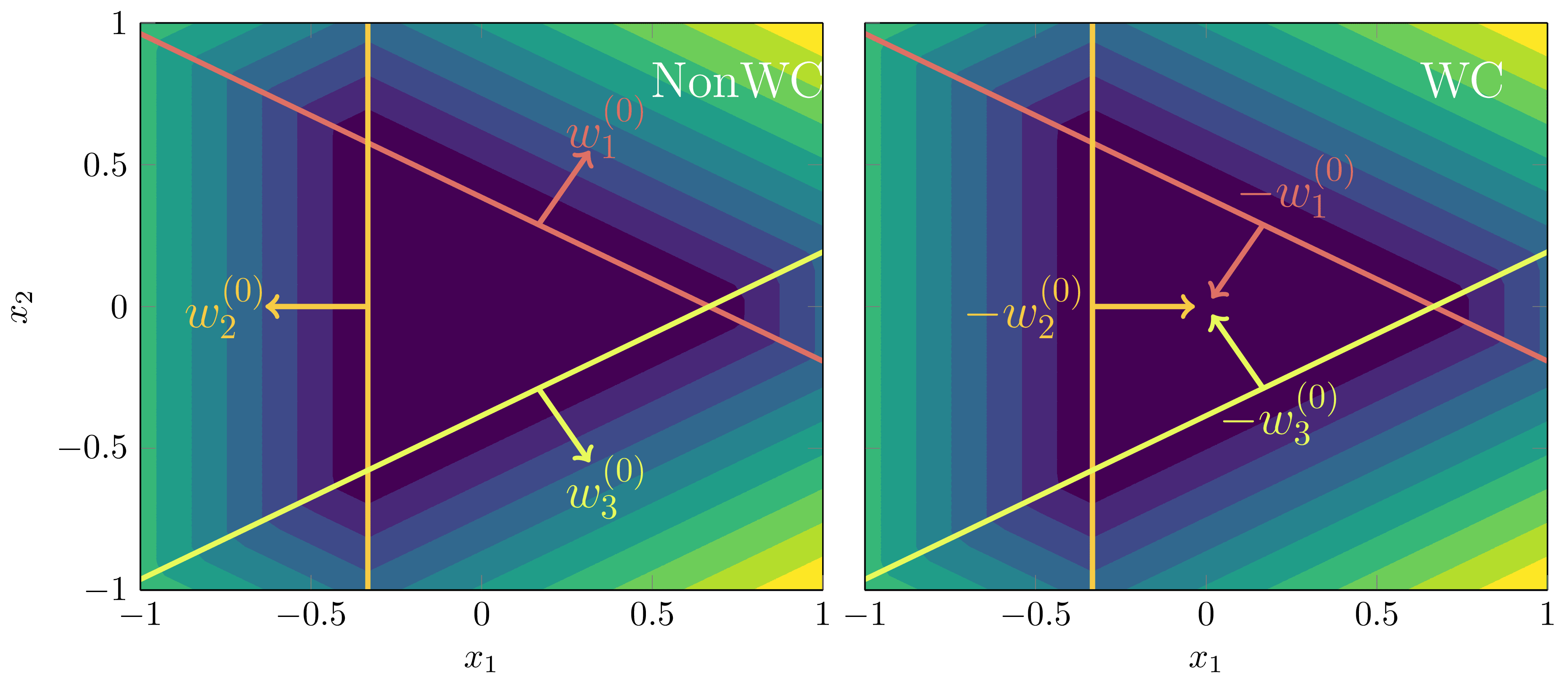
Example 3.3: Consider a true distribution defined by a (one-input) feedforward ReLU given by

$$\begin{array}{cc}{f}_0\left(x\right)& =ReLU(x-1)+ReLU(-x-1)+2\\ & =\{\begin{array}{cc}-x+1& x\le -1\\ 2& -1\le x\le 1\\ x+1& x\ge 1\end{array}\end{array}$$

where $w_1^{\left(0\right)}=1$, $w_2^{\left(0\right)}=-1$, and the activation boundaries are $H_1^{\left(0\right)}=\{x=1\}$ and $H_2^{\left(0\right)}=\{x=-1\}$.

Surprisingly, though it may appear our linear regions and activation boundaries must uniquely define the function (up to the scaling and permutation symmetries), there is a particular symmetry that arises by reversing the orientation of the weights and first layer biases, and adjusting the total bias accordingly. When we say reverse the orientation, we mean negating their direction,

$$w_1=-w_1^{\left(0\right)}=-1\text{and}{w}_2=-w_2^{\left(0\right)}=1,$$

and ditto for the biases. If we adjust the total bias $c$ accordingly, then following function

$$f(x,w)=ReLU(-x+1)+ReLU(x+1)$$

gives the same functional output!

Reversing the orientation of the true weights preserves this function because the true weights annihilate one another.

There is a very specific reason we can do this: in the middle region $-1\le x\le 1$, both nodes are active and cancel out to give a constant function,

$$f(x,w)=(-x+1)+(x+1)=2,$$

because the total gradients of the underlying truth sum to zero, $w_1^{\left(0\right)}+w_2^{\left(0\right)}=0$.

General case

Suppose the true network $f_0\left(x\right)$ is defined by a fixed $w^{\left(0\right)}=(w_1^{\left(0\right)},\dots ,b_1^{\left(0\right)},\dots q_1^{\left(0\right)},\dots ,c)$ for $m$ nodes. If there is a set $F\subseteq \left[m\right]$ of total gradients that sum to 0,

$$\sum _{i\in F}{q}_i^{\left(0\right)}{w}_i^{\left(0\right)}=0$$

then the model can produce functional equivalence by reversing the orientation of those particular weights (associated to those activation boundaries), biases, and adjusting the total bias. In other words, modulo permutation and scaling symmetry, there is a functionally equivalent network to $f_0\left(x\right)$ where the weights of every $i\in F$ satisfy

$$w_i=-w_i^{\left(0\right)}.$$

We call the condition ${\sum }_{i\in F}{q}_i^{\left(0\right)}{w}_i^{\left(0\right)}=0$ weight annihilation.

In [Carroll21, $\S$4.5] we define $m$-symmetric networks where the weights are progressive rotations by the angle $\frac{2\pi }{m}$, thus their total sum is zero. In DSLT4, we will study whether the posterior prefers configurations of weight-annihilation or not. (The answer is: not). ^[6]

An $m$-symmetric network for $m=3$ with $q_i^{\left(0\right)}=1$ and $c^{\left(0\right)}=0$. Both configurations, non-weight-cancellation (left) and weight-cancellation (right), are functionally equivalent since ${\sum }_{i=1}^3{w}_i^{\left(0\right)}=0$. Here, weight cancellation refers to the configuration where all three nodes are active in the central linear domain, but cancel to give an effective gradient of zero there.

Node Degeneracy

This is possibly the most important symmetry of all: neural network models can have more nodes than they need to represent a particular function. In essence, this degeneracy is the reason that different regions of the loss-landscape $K\left(w\right)$ of neural networks have fundamentally different accuracy-complexity tradeoffs. In other words, if the model has $d$ nodes in the hidden layer available to it, then all possible subnetwork configurations with less than $d$ nodes are also contained within the loss landscape. Thus, increasing the width of the network can only serve to increase the accuracy of these models, without sacrificing its ability to generalise, since the posterior will just prefer that number of hidden nodes with the best accuracy-complexity tradeoff.

Motivating Example

Example 3.4: Suppose we had a (one-input) true network given by

$$f_0\left(x\right)=ReLU\left(x\right)$$

and our model had $d=2$ nodes (with fixed biases $b_1=b_2=c=0$ and outgoing weights $q_1=q_2=1$),

$$f(x,w)=ReLU\left(w_{1}x\right)+ReLU\left(w_{2}x\right).$$

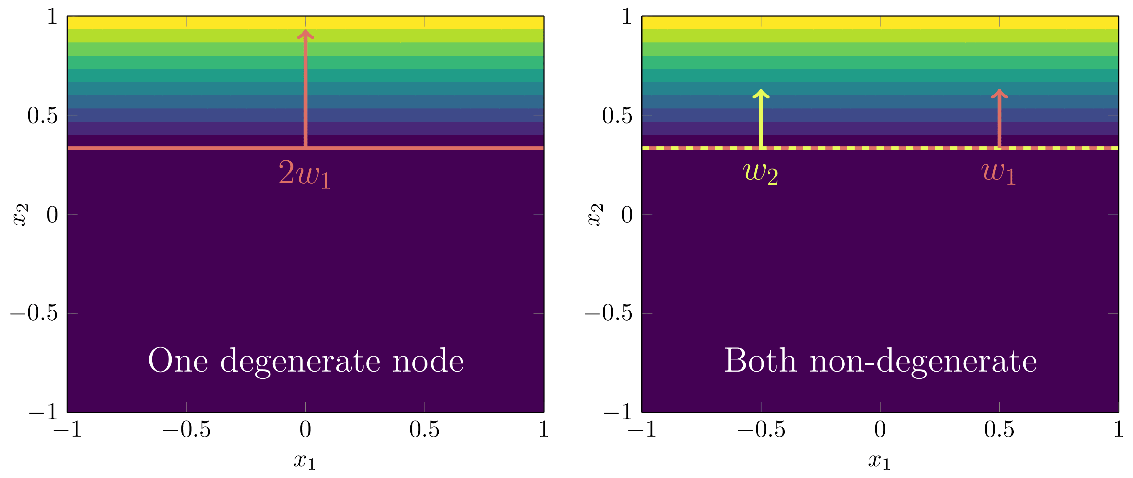
Since $f_0\left(x\right)=0$ for $x\le 0$, both weights must be positive, $w_1,w_2\ge 0$, to have any hope of being functionally equivalent. If $f(x,w)=f_0\left(x\right)$, we are in one of two configurations:

One node is degenerate: Either $(w_1,w_2)=(1,0)$ or $(w_1,w_2)=(0,1)$, meaning

$$f(x,w)=ReLU\left(1x\right)+ReLU\left(0x\right)=ReLU\left(x\right)=f_0\left(x\right).$$

Both nodes are non-degenerate, but the total gradient is the same as the truth: So long as the weights satisfy

$$w_1+w_2=1,$$

for $w_1,w_2>0$, we will have functional equivalence since, setting $w_2=1-w_1$,

$$\begin{array}{cc}f(x,w)& =ReLU\left(w_{1}x\right)+ReLU\left(\right(1-w_1\left)x\right)\\ & =\{\begin{array}{cc}{w}_{1}x+(1-w_1)x& x\ge 0\\ 0& x\le 0\end{array}\\ & =ReLU\left(x\right)\\ & =f_0\left(x\right).\end{array}$$

Node-degeneracies Correspond to Different Phases

We could of course encapsulate both of these configurations into the one statement that $w_1+w_2=1$ for $w_1,w_2\ge 0$, but there is a key reason we have delineated them: they represent two different phases and have different geometry on $K\left(w\right)$. Intuitively, the degenerate phase is a simpler model with less complexity, thus we expect it has a lower RLCT ^[7], and for the posterior to prefer it. In DSLT4 we will discuss phases in statistical learning more broadly, and display experimental evidence for this latter claim.

To foreshadow this, we can actually calculate $K\left(w\right)$ for Example 3.4. Setting the prior $q\left(x\right)$ to be uniform on $[-\sqrt{6},\sqrt{6}]$ we find

$$K(w_1,w_2)=\{\begin{array}{cc}(w_1+w_2-1{)}^2& w_1,w_2\ge 0\\ w_1^2+(w_2-1{)}^2& w_1\le 0,w_2\ge 0\\ (w_1-1{)}^2+w_2^2& w_1\ge 0,w_2\le 0\\ (w_1+w_2{)}^2+1& w_1,w_2\le 0\end{array}.$$

$K\left(w\right)$ for the above example with slightly wider bowls at the degenerate-node phases.

Notice how there are ever so slightly wider bowls at either end of the line $w_1+w_2=1$, thus suggesting the posterior has more density at the degenerate phase $(w_1,w_2)=(0,1)$(or vice versa). Intuitively, imagine a tiny ball being with random kinetic energy rolling around the bottom of the surface—it will spend more time in the ends since there is more catchment area. (Don’t take the physics analogy too seriously, though).

We see once again that the singularity structure of the minima has a big impact on the geometry of $K\left(w\right)$, and therefore the posterior.

General Case

Suppose we have a truth $f_0\left(x\right)$ and model $f(x,w)$ that are both defined by two layer feedforward ReLU neural networks, where the model has $d$ nodes and the truth has $m$ nodes (assumed to all be non-degenerate and with distinct activation boundaries) such that $m<d$. Then the model is overparameterised compared to the truth it is trying to model.

Performing the appropriate analysis (which we do in Appendix 2), one finds that:

1. Without loss of generality (i.e. up to permutation symmetry), the first $m$ nodes of $\left[d\right]$ must have the same activation boundaries as those in $f_0\left(x\right)$, and satisfy the same scaling, permutation and orientation reversing symmetries as discussed above.

2. For the remaining nodes $i\in \{m+1,\dots ,d\}$ of the model, each one either:

   • Is degenerate, so $w_i=0$ or $q_i=0$, or;

   • Shares the same activation boundary as one already in $\left[m\right]$ such that the total gradients sum to the correct gradient in each region. (In our above example, this is saying that necessarily $w_1+w_2=1$ since these nodes share the same activation boundary).

The function $f_0\left(x\right)=2ReLU(x_2-\frac{1}{3})$ can also be represented by a two node model where both nodes share the same boundary, $f(x,w)=ReLU(x-\frac{1}{3})+ReLU(x-\frac{1}{3})$.

In DSLT4 we will test which of the phases in the above figure is preferred by the posterior for this simple two layer feedforward ReLU neural networks setup.

Node degeneracy is the same as lossless network compressibility

The fact that neural networks can contain these node-degeneracies is well known and often goes under the guise of lossless network compressibility. There are many notions of compressibility, but the one that makes the most sense in our setup is to say that if the model has $d>m$ hidden nodes compared to the truth, then it can be compressed to a network with only $m$ hidden nodes and still produce the same input-output map.

For an excellent introduction to lossless network compressibility, see Farrugia-Roberts’ recent paper Computational Complexity of Detecting Proximity to Losslessly Compressible Neural Network Parameters, where he studies the problem for $\tanh$networks.

There are More True Parameters if the Input Domain is Bounded

Let me make an important remark here. In both of the above cases, we have considered the symmetries of $W_0$ when the input domain of the model and the truth is all of $R^2$. As we explain in Appendix 2, this allows us to compare the gradients and biases of hyperplanes, similar to comparing polynomial coefficients, to make our conclusions. However, if the domain of the input prior $q\left(x\right)$ is restricted to some open bounded domain $Z\subseteq R^2$, there could in principle be more degeneracies and symmetries of $W_0$, since the functional equivalence only needs to be on $Z$.

For example, consider a true network defined by $f_0\left(x\right)=0$ and a single-node single-input model $f(x,w)=qReLU(⟨w,x⟩+b)$ defined on $Z=(-a,a)$, so $q\left(x\right)=\frac{1}{2a}1(-a<x<a)$. If the activation boundary falls outside of $Z$ and the vector $w$ points away from $Z$, then any value of $q,w,b$ satisfying these constraints would give $f(x,w)=0$, thus there is an entirely new class of symmetry in $W_0$.

Whilst important to keep this mind, we won’t discuss this any further as it opens up an entirely different can of worms.

Even if Singularities Occur with Probability Zero, they Affect Global Behaviour in Learning

I want to make a quick comment on the work of Phuong and Lampert in [PL19]. In this paper, they prove equivalent results to these for arbitrary depth feedforward ReLU neural networks (with non-increasing widths), but with a key distinction: they consider general models. In their words,

A sufficient condition for a network to be general with probability one is that the weights are sampled from a distribution with a density.

They then show that almost all feedforward ReLU networks with this architecture are general, and then show that general networks only satisfy scaling and permutation symmetries, thus excluding our orientation-reversing and degenerate node singularities since they occur on a set of measure zero. Importantly, this implies that almost all parameters $w\in W$ have no degenerate nodes, or equivalently, no opportunity for lossless compression.

However, even though scaling and permutation symmetries may be the only generic symmetries (in the sense of measure theory) that occur with non-zero probability, SLT tells us that the singularities of $K\left(w\right)$ have global effects on the loss landscape, as we discussed at length in DSLT2. If a parameter is near a non-generic singularity (i.e. one that occurs with probability zero), it computes a function that is almost identical to the one computed by that of a non-generic singularity. If we shift our language to that of compressibility of a network, SLT tells us that:

Just because a particular point $w\in W$ sampled from a posterior (or, notionally, obtained via running SGD) is not directly compressible itself, that doesn’t mean that it isn’t extremely close to one that is.

In this sense, SLT tells us that to understand the geometry of the loss landscape, we need to consider singularities even though they are not generic points. As Watanabe says, singularities contain knowledge.

Appendix 1 - Formal Proof that Neural Networks are Singular

If, like me, you are mathematically inclined, you probably want to see a proof that these neural networks are, indeed, singular models, to tie together the various concepts and intuitions that we have built in this sequence so far. So let’s turn into math mode briefly.

Recall that the Fisher information matrix $I\left(w\right)$ is degenerate if and only if the set

$${\left\{\frac{\partial }{\partial w_j}f\right(x,w\left)\right\}}_{j=1}^D$$

is linearly dependent. Here, $\frac{\partial }{\partial w_j}$ refers to the partial derivative with respect to the $j$th component of the total parameter $w\in W$, not to be confused with the specific weight vector $w_j$ in the neural network definition. Thus, to prove that feedforward ReLU networks are singular, our task is to find this linear dependence relation. The scaling symmetry alone is enough for this.

Theorem: Given a two layer feedforward neural network $f:R^2\times W\to R$ with $d$ hidden nodes, for any domain on which $f$ is differentiable, $f$ satisfies the differential equation for a fixed node $i\in \left[d\right]$:

$$\{w_{i,1}\frac{\partial }{\partial w_{i,1}}+w_{i,2}\frac{\partial }{\partial w_{i,2}}+b_i\frac{\partial }{\partial b_i}-q_i\frac{\partial }{\partial q_i}\}f=0.$$

Proof: Since $\frac{d}{dx}ReLU\left(x\right)=1\{x>0\}$, and letting $a_i=⟨w_i,x⟩+b_i$, the set of derivatives with respect to our parameters are

$$\frac{\partial f}{\partial w_{1,k}}=q_1{x}_{k}1(a_i>0),\frac{\partial f}{\partial b_i}=q_{1}1(a_i>0),\frac{\partial f}{\partial q_i}=ReLU\left(a_i\right),$$

and so since we can write $ReLU\left(a_i\right)=a_{i}1(a_i>0)$ we have

$$\begin{array}{cc}& \{w_{i,1}\frac{\partial }{\partial w_{i,1}}+w_{i,2}\frac{\partial }{\partial w_{i,2}}+b_i\frac{\partial }{\partial b_i}-q_i\frac{\partial }{\partial q_i}\}f\\ & =q_i{w}_{i,1}{x}_{1}1(a_i>0)+q_i{w}_{i,2}{x}_{2}1(a_i>0)+q_i{b}_{i}1(a_i>0)-q_{i}ReLU\left(a_i\right)\\ & =q_{i}ReLU(⟨w_i,x⟩+b_i)-q_{i}ReLU(⟨w_i,x⟩+b_i)=0.\square \end{array}$$

Corollary: Feedforward ReLU neural networks are singular models.

Proof: For the two layer case, for any fixed $w^0\in W$, there is a linear dependence relation given by the above differential equation evaluated at $w^0$, thus the Fisher information is degenerate at $w^0$, so the model is singular.

The equivalent proof for arbitrary depths and widths is given in Lemma A.1 of [Wei22], following from other work on functional equivalence in [PL19]. $\square$

The degenerate node symmetries also give rise to a degenerate Fisher information matrix, though I haven’t formally written out this alternate proof yet. If you are interested, do it as an exercise and leave it as a comment!

Appendix 2 - Proof Sketch for Fully Classifying $W_0$ for Two Layer Feedforward ReLU Networks

This section is going to be slightly more technical, and in the grand scheme of the SLT story I am telling in this sequence, this may be seen as an unnecessary side-plot. But, other readers, particularly those with a pure mathematical bent, may find it interesting to consider the process of fully classifying $W_0$ and how one might understand all phases present, so I am providing a sketch of these proofs for completeness. Understanding the full form of $W_0$ was a vital part of performing the phase transition experiments that we will see in DSLT4. These models are simple enough that we can perfectly classify all true parameters in $W_0$. Thus, we can precisely understand all of its phases.

We are going to classify the symmetries of $W_0$ when both the model $f(x,w)$ and truth $f_0\left(x\right)$ are two-layer feedforward ReLU neural networks, with $d$ and $m$ hidden nodes respectively, giving

$$W_0=\{w\in W|f(x,w)=f_0(x\left)\right\},$$

meaning the task is to classify functional equivalence of the two networks. To avoid some annoying fringe cases, we assume that the true network is minimal, which means there is no network with fewer nodes that could also represent it (which also means every node is non-degenerate), and activation-distinguished, meaning every node of the truth corresponds to a unique activation boundary.

We will see that the set of symmetries explained above comprise all of the symmetries in $W_0$ - there can be no more ^[8]. This result rests mainly on the fact that the activation boundaries are the core piece of data that defines a neural network. The rest is then just performing accounting of the gradients and biases in each region.

This is a sketch of the proofs in Chapter 4 of my thesis, and all lemmas and theorems that are referenced in the following section come from here.

Case 1: The model has the same number of nodes as the truth, $m=d$

Let $f(x,w)$ be a two layer feedforward ReLU neural network model with $d$ hidden nodes, and let $f_0\left(x\right)=f(x,w^{\left(0\right)})$ be the realisable true network with $m$ hidden nodes defined by a fixed parameter $w^{\left(0\right)}$, denoted by

$$f_0\left(x\right)=c^{\left(0\right)}+\sum _{j=1}^m{q}_i^{\left(0\right)}ReLU(⟨w_j^{\left(0\right)},x⟩+b_j^{\left(0\right)}),$$

which we assume is minimal and activation-distinguished as explained above.

We start by comparing the foldsets, which are the activation boundaries [Lemma 4.1], between the truth and the model. Let $H_i$ be the activation boundary of the node $i\in \left[d\right]$ in the model, and $H_j^{\left(0\right)}$ be the activation boundary of the node $j\in \left[m\right]$ in the truth. Then by comparing the sets of linear lines in [Lemma 4.2], we can show that for every node of the model $i\in \left[d\right]$ there exists a permutation $\sigma \in S_m$ such that

$$H_i=H_{\sigma \left(i\right)}^{\left(0\right)}.$$

By [Lemma 4.3], two activation boundaries $H,H^{\prime }$ are equal if and only if there is some non-zero scalar $\alpha \in R\setminus \left\{0\right\}$ such that $w=\alpha w^{\prime }$ and $b=\alpha b^{\prime }$.

Using our relation $H_i=H_{\sigma \left(i\right)}^{\left(0\right)}$, in [Lemma 4.4] we analyse how the gradients and biases change across each activation boundary, and what this means for the relation between weights and biases in the model versus the truth. We show that there exists a unique $\sigma \in S_m$, and for each $i\in \left[d\right]$ an ${ϵ}_i\in Z_2$ and ${\alpha }_i\in R_{>0}$ such that

$$w_i=(-1{)}^{{ϵ}_i}{\alpha }_i{w}_{\sigma \left(i\right)}^{\left(0\right)},\text{and}{b}_i=(-1{)}^{{ϵ}_i}{\alpha }_i{b}_{\sigma \left(i\right)}^{\left(0\right)},\text{where}{\alpha }_i=\frac{q_{\sigma \left(i\right)}^{\left(0\right)}}{q_i},$$

meaning $q_i$ and $q_{\sigma \left(i\right)}^{\left(0\right)}$ necessarily have the same sign.

However, there is a restriction on which weights can have reversed orientation, ${ϵ}_i=1$ (thus $w_i=-{\alpha }_i{w}_{\sigma \left(i\right)}^{\left(0\right)}$). Letting $E=\{i\in [d]|{ϵ}_i=1\}$, we show in [Lemma 4.5] that the weights and biases of the true network must satisfy ^[9]

$$\sum _{i\in E}{q}_{\sigma \left(i\right)}^{\left(0\right)}{w}_{\sigma \left(i\right)}^{\left(0\right)}=0\text{and}{c}^{\left(0\right)}+\sum _{i\in E}{q}_{\sigma \left(i\right)}^{\left(0\right)}{b}_{\sigma \left(i\right)}^{\left(0\right)}=c.$$

The crux of this proof rests in comparing the gradients in regions either side of the activation boundary $H_i$.

In [Theorem 4.7] we show that these scaling, permutation and orientation reversing symmetries are the only such symmetries by piecing together all of these aforementioned Lemmas, with emphasis on the importance of the activation boundaries in defining the topology of $f_0\left(x\right)$. ^[10]

Case 2: The model has more nodes than the truth, $m<d$

We now suppose that the model is over-parameterised compared to the true network, so $m<d$.

The key piece of data is once again the foldsets defining the model and the truth. Since they must be equal, the model can only have $m$ unique foldsets, and thus activation boundaries. Without loss of generality (i.e. up to permutation symmetry), the first $\left[m\right]\subset \left[d\right]$ nodes in the model have the same activation boundaries as the truth, ${\bigcup }_{i=1}^m{H}_i={\bigcup }_{j=1}^m{H}_j^{\left(0\right)}$. Thus, these $\left[m\right]$ nodes in the model must satisfy the same symmetries as in the $m=d$ case.

By comparing the fold sets on each excess node in $\{m+1,\dots ,d\}$, we must have

$$\bigcup _{i=m+1}^d\left\{H_i|i\text{is non-degenerate}\right\}\subseteq \bigcup _{j=1}^m{H}_j^{\left(0\right)}.$$

In comparing linear lines again, this means there are two possible situations:

1. $\left\{H_i|i\text{is non-degenerate}\right\}$ is empty, so node $i$ is degenerate, meaning $q_i=0$ or $w_i=0$, or;

2. $H_i=H_j^{\left(0\right)}$ for some $j\in \left[m\right]$, so node $i$ shares an activation boundary already in the first $\left[m\right]$ nodes of the model.

Let $d^{\prime }\ge m$ the number of non-degenerate nodes of the model. We can thus define a surjective finite set map

$$\pi :\{1,\dots ,m,m+1,\dots ,d^{\prime }\}\to \{1,\dots ,m\}$$

relating the non-degenerate nodes in the model to those in the truth, which is a bijection (i.e. a permutation $\sigma \in S_m$) on the first $\left[m\right]\subset \left[d^{\prime }\right]$.

We can then compare the gradients and biases in each region to show that the total gradients calculated by each non-degenerate node at each unique activation boundary must sum to the gradient in the truth. Precisely, for each node $j\in \left[m\right]$ of the truth, let $M_j=\{i\in [d^{\prime }\left]|\pi \right(i)=j\}$ be the set of nodes in the model that share the same activation boundary. Then for each $i\in \left[d^{\prime }\right]$ there exists an ${ϵ}_i\in Z_2$ and ${\alpha }_i\in R_{>0}$ such that

$$w_i=(-1{)}^{{ϵ}_i}{\alpha }_i{w}_{\pi \left(i\right)}^{\left(0\right)},b_i=(-1{)}^{{ϵ}_i}{\alpha }_i{b}_{\pi \left(i\right)}^{\left(0\right)}$$

with the constraint that

$$\sum _{i\in M_j}{q}_i{\alpha }_i=q_j^{\left(0\right)}.$$

A similar orientation reversing symmetry also applies as in case 1, just by accounting for the nodes that share the same activation boundaries.

Resources

[Carroll21] - L. Carroll, Phase Transitions in Neural Networks, 2021

[Wei22] - S. Wei, D. Murfet, et al., Deep Learning is Singular, and That’s Good, 2022

[PL19] - M. Phuong, C. Lampert, Functional vs Parametric Equivalence of ReLU networks, 2019

---

1. ^

   Since $K\left(w\right)=0$ if and only if $q\left(y|x\right)=p(y|x,w)$ for some $w\in W$.

2. ^

   e.g. $ReLU\left(x\right)+ReLU\left(x\right)=ReLU\left(2x\right)$. ↩︎

3. ^

   For ease of classification, we exclude the case where $q_i\ne 0$ and $b_i\ne 0$ since we can just absorb the total bias contribution into $c$. ↩︎

4. ^

   A linear domain $U\subseteq R^2$ is just a connected open set where $f_w$ is a plane with constant gradient and bias when restricted to $U$, and $U$ is the maximal such set for which that plane is defined. In other words, the set of linear domains are the set of different regions the piecewise affine function are carved up into. ↩︎

5. ^

   But don’t forget, $ReLU(-x)\ne -ReLU\left(x\right)$ as the domain of activation is completely different. ↩︎

6. ^

   Though I have not been able to formally prove it, I believe that this symmetry on its own (i.e. modulo scaling symmetry) does not result in a degeneracy of the Fisher information matrix, at least in our simple case. This, I think, is because the weights must cancel out in the region where both nodes are active, and the gradients in the other regions must be retained. Feel free to prove me wrong, though! ↩︎

7. ^

   This statement is a bit disingenuous. Watanabe’s free energy formula only applies to the case where $K\left(w\right)$ is analytic, but ReLU neural networks are certainly not analytic, as we can see in the below example. With that said, Watanabe has recently proved a bound on the free energy for ReLU neural networks, showing that the complexity term is essentially related to the number of non-degenerate nodes in the truth, even if it isn’t a true RLCT. We will look at this in more depth in DSLT4. ↩︎

8. ^

   Aside from the technical caveat discussed about the restricted input prior $q\left(x\right)$ above.

9. ^

   Our convention is to take the empty sum to be 0, so all weight orientations being preserved, $E=\varnothing$, is perfectly fine. ↩︎

10. ^

    The activation distinguished condition on the truth allows us to uniquely identify the permutation $\sigma \in S_m$ relating activation boundaries, and ensures only one node changes across each boundary. ↩︎

[lsgos]

I’m trying to read through this more carefully this time: how load-bearing is the use of ReLU nonlinearities in the proof? This doesn’t intuitively seem like it should be that important (e.g a sigmoid/​gelu/​tanh network feels like it is probably singular, and it certainly has to be if SLT is going to tell us something important about NN behaviour because changing the nonlinearity doesn’t change how NNs behave that much imo), but it does seem to be an important part of the construction you use.

[Liam Carroll]

Good question! The proof of the exact symmetries of this setup, i.e. the precise form of $W_0$, is highly dependent on the ReLU. However, the general phenomena I am discussing is applicable well beyond ReLU to other non-linearities. I think there are two main components to this:

1. Other non-linearities induce singular models. As you note, other non-linear activation functions do lead to singular models. @mfar did some great work on this for tanh networks. Even though the activation function is important, note that the better intuition to have is that the hierarchical nature of a model (e.g. neural networks) is what makes them singular. Deep linear networks are still singular despite an identity activation function. Think of the activation as giving the model more expressiveness.

2. Even if $W_0$ is uninteresting, the loss landscape might be “nearly singular”. The ReLU has an analytic approximation, the Swish function ${\sigma }_{\beta }\left(x\right)=\frac{x}{1+e^{-\beta x}}$, where ${lim}_{\beta \to \infty }{\sigma }_{\beta }\left(x\right)=ReLU\left(x\right)$, which does not yield the same symmetries as discussed in this post. This is because the activation boundaries are no longer a sensible thing to study (the swish function is “always active” in all subsets of the input domain), which breaks down a lot of the analysis used here.
   
   Suppose, however, that we take a ${\beta }_0$ that is so large that from the point of view of your computer, ${\sigma }_{{\beta }_0}\left(x\right)=ReLU\left(x\right)$ (i.e. their difference is within machine-epsilon). Even though $W_0^{\text{swish}}$ is now a very different object to $W_0^{\text{ReLU}}$ on paper, the loss landscape will be approximately equal $L_{\text{swish}}\left(w\right)\approx L_{\text{ReLU}}\left(w\right)$, meaning that the Bayesian posterior will be practically identical between the two functions and induce the same training dynamics.
   
   So, whilst the precise functional-equivalences might be very different across activation functions (differing $W_0$), there might be many approximate functional equivalences. This is also the sense in which we can wave our arms about “well, SLT only applies to analytic functions, and ReLU isn’t analytic, but who cares”. Making precise mathematical statements about this “nearly singular” phenomena—for example, how does the posterior change as you lower $\beta$ in ${\sigma }_{\beta }\left(x\right)$? - is under-explored at present (to the best of my knowledge), but it is certainly not something that discredits SLT for all of the reasons I have just explained.

[lsgos]

Yeah I agree with everything you say; it’s just I was trying to remind myself of enough of SLT to give a a ‘five minute pitch’ for SLT to other people, and I didn’t like the idea that I’m hanging it of the ReLU.

I guess the intuition behind the hierarchical nature of the models leading to singularities is the permutation symmetry between the hidden channels, which is kind of an easy thing to understand.

I get and agree with your point about approximate equivalences, though I have to say that I think we should be careful! One reason I’m interested in SLT is I spent a lot of time during my PhD on Bayesian approximations to NN posteriors. I think SLT is one reasonable explanation of why this. never yielded great results, but I think hand-wavy intuitions about ‘oh well the posterior is probably-sorta-gaussian’ played a big role in it’s longevity as an idea.

yeah it’s not totally clear what this ‘nearly singular’ thing would mean? Intuitively, it might be that there’s a kind of ‘hidden singularity’ in the space of this model that might affect the behaviour, like the singularity in a dynamic model with a phase transition. but im just guessing

[Leon Lang]

Thanks Liam also for this nice post! The explanations were quite clear.

The property of being singular is specific to a model class $f(x,w)$, regardless of the underlying truth.

This holds for singularities that come from symmetries where the model doesn’t change. However, is it correct that we need the “underlying truth” to study symmetries that come from other degeneracies of the Fisher information matrix? After all, this matrix involves the true distribution in its definition. The same holds for the Hessian of the KL divergence.

Both configurations, non-weight-annihilation (left) and weight-annihilation (right)

What do you mean with non-weight-annihilation here? Don’t the weights annihilate in both pictures?

[Liam Carroll]

However, is it correct that we need the “underlying truth” to study symmetries that come from other degeneracies of the Fisher information matrix? After all, this matrix involves the true distribution in its definition. The same holds for the Hessian of the KL divergence.

The definition of the Fisher information matrix does not refer to the truth $q(y,x)$ whatsoever. (Note that in the definition I provide I am assuming the supervised learning case where we know the input distribution $q\left(x\right)$, meaning the model is $p(y,x|w)=p(y|x,w)q\left(x\right)$, which is why the $q\left(x\right)$ shows up in the formula I just linked to. The derivative terms do not explicitly include $q\left(x\right)$ because it just vanishes in the $w_j$ derivative anyway, so its irrelevant there. But remember, we are ultimately interested in modelling the conditional true distribution $q\left(y|x\right)$ in $q(y,x)=q\left(y|x\right)q\left(x\right)$.)

What do you mean with non-weight-annihilation here? Don’t the weights annihilate in both pictures?

You’re right, thats sloppy terminology from me. What I mean is, in the right hand picture (that I originally labelled WA), there is a region in which all nodes are active, but cancel out to give zero effective gradient, which is markedly different to the left hand picture. I have edited this to NonWC and WC instead to clarify, thanks!