DSLT 4. Phase Transitions in Neural Networks

[Liam Carroll]

TLDR; This is the fourth main post of Distilling Singular Learning Theory which is introduced in DSLT0. I explain how to relate SLT to thermodynamics, and therefore how to think about phases and phase transitions in the posterior in statistical learning. I then provide intuitive examples of first and second order phase transitions in a simple $K\left(w\right)$ loss function. Finally, I experimentally demonstrate phase transitions in two layer ReLU neural networks associated to the node-degeneracy and orientation-reversing phases established in DSLT3, which we can understand precisely through the lens of SLT.

In deep learning, the terms “phase” and “phase transition” are often used in an informal manner to refer to a steep change in a metric we care about, like the training or test loss, as a function of SGD steps, or alternatively some hyperparameter like the number of samples from the truth $n$.

A classic example of a phase transition in deep learning literature is Anthropic’s Induction Heads paper, where the “bump” in loss (in-context learning score) is referred to as a “phase change”.

But what exactly are the phases? And why do phase transitions even occur? SLT provides us a solid theoretical framework for understanding phases and phase transitions in deep learning. In this post, we will argue that in the Bayesian setting,

A phase of the learning process corresponds to a singularity of $K\left(w\right)$, and a phase transition corresponds to a drastic change in the posterior as a function of a hyperparameter $\theta$.

The hyperparameter $\theta$ could be the number of samples from the truth $n$, some way of varying the model function $f(x,w)=f(x,w;\theta )$ or something about the true distribution $D_n=D_n\left(\theta \right)$, amongst other things. At some critical value $\theta ={\theta }_c$, we recognise a phase transition as being a discontinuous change in the free energy or one of its derivatives, for example the generalisation error $G_n=E\left[F_{n+1}\right]-E\left[F_n\right]$.

In this post, we will present experiments that observe precise phase transitions in the toy neural network models we studied in DSLT3, for which we understand the set of true parameters $W_0$ and therefore the phases. By the end of this post, you will have a framework for thinking about phase transitions in singular models and an intuition for why SLT predicts them to occur in learning.

Phases Correspond to Singularities

The Story Starts in Physics

This subsection is modelled on [Callen, Ch9], but it is only intended to be a high level discussion of the concepts grounded in some basic physics—don’t get too bogged down in the details of the thermodynamics.

Fundamentally, a phase describes an aggregate state of a complex system of many interacting components, where the state retains particular qualities with variations in some hyperparameter. To explain the concept in detail, it is natural to start in physics (thermodynamics in particular), where these ideas originally arose. But there is a deeper reason to build from here: every human has an intuitive understanding of the phases of water and how they change with temperature ^[1], which serves as the base mental model for what a phase is.

One of the main goals of thermodynamics is to study how the equilibrium state of a system changes as a function of macroscopic parameters. In the case of a vessel of water at 1atm of pressure in constant contact with a thermal and pressure reservoir, the equilibrium state of the system corresponds to a state that is minimised by the Gibbs free energy $F$ ^[2]. The phases, then, are the equilibrium states, which describe qualitative physical properties of the system. The states of matter—solid, liquid, and gas—are all phases of water, which are characterised by variables like their volume and crystal structure. As anybody that has boiled water before knows, these phases undergo transitions as a function of temperature. Let’s make this more precise.

The Thermodynamic Setup

Consider a system of $K$ water molecules moving in a 2D container, each with equal mass $m$. To each particle $i\in \left[K\right]=\{1,\dots ,K\}$ we can associate a set of microstates describing its physical properties at a point in time, for example its position $x_i$ and its velocity $v_i$. In our discussion we will simply focus on the position, which we will relabel $w=(w_1,\dots ,w_K)$ (for reasons that will become clear), so our configuration space $W\subseteq R^{2K}$ of possible microstates is

$$W=\left\{w|\right(w_{i,x},w_{i,y})\in R^2\text{for each}i\in [K\left]\right\}.$$

Since it is physically infeasible to know or model the positions of all molecules, we instead reason about the dynamics of the system by calculating macroscopic variables associated to a microstate, for example the temperature or total volume of the molecules. We will focus on the volume $V\left(w\right)$ of a microstate $w$. Importantly, a macroscopic state is an aggregate over the system (for example, temperature being related to average squared velocity), meaning there are many possible configurations of microstates that result in the same macrostate. To this end, we can define regions of our configuration space according to their volume $v$,

$$W_v=\{w\in W|V(w)=v\}\subseteq W.$$

In our toy example, we want to study how the system changes as a function of temperature, which we will denote with $\theta$. In a Gibbs ensemble, we can associate an energy functional, the Hamiltonian $H(w;\theta )$, to any given microstate $w$ at temperature $\theta$. The fundamental postulate of such a Gibbs ensemble is that probability of the system being in a particular micro state $w$ is determined by a Gibbs distribution ^[3]

$$p(w;\theta )=\frac{e^{-H(w;\theta )}}{Z}\text{where}Z={\int }_W{e}^{-H(w;\theta )}dw.$$

This should look pretty familiar from our statistical learning setup! Indeed, we can then calculate the free energy of the ensemble for different volumes $v$ at temperature $\theta$,

$$F_{\theta }\left(v\right)=-\log \left({\int }_{W_v}{e}^{-H(w;\theta )}dw\right).$$

For a Gibbs ensemble, the equilibrium state of a given system is that state which minimises the free energy. In the context of bringing water to a boiling point, there are two minima of the free energy characterised by the liquid and gaseous states, which for ease we will characterise by their volumes $v_{\text{liquid}}$ and $v_{\text{gas}}$. Then the equilibrium state changes at the critical temperature ${\theta }_c=100°C$,

$$\{\begin{array}{cc}{W}_{v_{\text{liquid}}}& 0°C<\theta <100°C\\ W_{v_{\text{gas}}}& \theta >100°C\end{array}.$$

Importantly, while small variations in the temperature away from ${\theta }_c$ will change the free energy of each state, it will not change the configuration of these minima with respect to the free energy. In other words, the system will still be a liquid for any $\theta \in (0,100)$ - its qualitative properties are stable. This is the content of a phase.

What is a phase?

A phase of a system is a region of configuration space $W\subset W$ that minimises the free energy, and is invariant to small perturbations in a relevant hyperparameter $\theta$. Typically, phases are distinguished by some macroscopic variable, in our case the volume $V\left(w\right)$ distinguishing subsets $W_v$. More generally though, a phase describes some qualitative aggregate state of a system—like, as we’ve discussed in our example, the states of matter.

Phases are minima of the free energy that remain minima with small perturbations in $\theta$.

In some sense, you can define a phase to be any region that induces an equilibrium state with qualities you care about. But what makes phases a powerful concept is their relation to phase transitions—when there is a sudden jump in which state is preferred by the system.

What is a phase transition?

Phase transitions are changes in the structure of the global minima of the free energy, and often arise as non-analyticities of $F_n$. This is a fancy way of saying they correspond to discontinuities in the free energy or one of its derivatives ^[4].

A first order phase transition at a critical temperature ${\theta }_c$ corresponds to a reconfiguration of which phase is the global minima of the free energy.

A first order phase transition exchanges global and local minima, changing the configuration of which phase is preferred according to which has the lowest free energy. These curves depict the phase transition as water reaches boiling point $\theta =100°C$.

As we discussed above, heating water to boiling point ${\theta }_c=100°C$ is a classic example of a first order phase transition.

Two examples of second order phase transitions are where:

• A merge transition occurs at ${\theta }_c$ when two phases that are initially disjoint for $\theta <{\theta }_c$ merge to become the same state for $\theta \ge {\theta }_c$, or;

• A creation transition occurs at ${\theta }_c$ when a local minima exists for $\theta \ge {\theta }_c$ but does not exist for $\theta <{\theta }_c$. (If the directions are reversed, we call this a destruction transition).

A second order merge phase transition (left), and a second order creation phase transition (right).

(Note that we have not given a full classification of phase transitions here, because to do so one needs to study the possible types of catastrophes that can occur, as presented in [Gilmore]).

Phases in Statistical Learning

The notation and concepts in the previous section were not presented without reason. For starters, the Gibbs ensemble view of statistical learning is actually quite a rich analogy because, when the prior is uniform, the (random) Hamiltonian is equal to the empirical KL divergence ^[5],

$$H_n\left(w\right)=n{K}_n\left(w\right).$$

The configuration space of microstates of the physical system then corresponds to parameter space $W$ with microstates given by different parameters $w\in W$. This means the posterior is equivalent to the Gibbs probability distribution of the system being in a certain microstate, meaning the definition of free energy is identical. So, what exactly are the phases then?

In statistical learning then,

A phase corresponds to a local neighbourhood $W\subset W$ containing a singularity $w_W^{\left(0\right)}$ of interest.

To say that $W$ minimises the free energy is equivalent to saying that it has non-negligible posterior mass. The reason for this, as we explored in DSLT2, is that the singularity structure of a most singular optimal point $w_W^{\left(0\right)}\in W_{\text{opt}}$ dominates the behaviour of the free energy, because it minimises the loss $L\left(w\right)$ and has the smallest RLCT ${\lambda }_W$.

You can, in principal, define a phase to be any region of $W$. But the analysis of phases in the posterior only gets interesting when you have a set of phases that have fundamentally different geometric properties. The free energy formula tells us that these geometric properties correspond to different accuracy-complexity tradeoffs.

Consequently, in statistical learning, Watanabe states in [Wat18, $\S 9.4$] that

A phase transition is a drastic change in the geometry of the posterior as a function of a hyperparameter $\theta$.

Our definitions of first and second order phase transitions carry over perfectly from the physics discussion above.

It’s important to clarify here that phase transitions in deep learning have many flavours. If one believes that SGD is effectively just “sampling from the posterior”, then the conception that phase transitions are related to changes in the geometry of the posterior carries over. There is, however, one fundamentally different kind of “phase transition” that we cannot explain easily with SLT: a phase transition of SGD in time, i.e. the number gradient descent steps. The Bayesian framework of SLT does not really allow one to speak of time—the closest quantity is the number of datapoints $n$, but these are not equivalent. We leave this gap as one of the fundamental open questions of relating SLT to current deep learning practice. ^[6]

The hyperparameter $\theta$ can affect any number of objects involved in the posterior. Remembering that the posterior is

$$p\left(w|D_n\right)=\frac{\phi \left(w\right)e^{-n{L}_n\left(w\right)}}{Z_n},$$

we could include hyperparameter $\theta$ dependence in any of:

• The model function $f(x,w)=f(x,w;\theta )$ (i.e. the neural network defining $p(y|x,w)).$

• The true distribution $D_n=D_n\left(\theta \right)$, meaning $L_n\left(w\right)=L_n(w;\theta )$. (This could in principal be dependence in the input prior $q\left(x\right)$ or the actual dataset generated by $q\left(y|x\right)$.)

• The number of datapoints $n$ (inducing a first order phase transition due to the change in accuracy-complexity tradeoff).

• The prior $\phi \left(w\right)=\phi (w;\theta )$.

Intuitive Examples to Interpret Phase Transitions

In DSLT2 we studied an example of a very simple one-dimensional $K\left(w\right)$ curve and got a feel for how the accuracy and complexity of a singularity affect the free energy of different neighbourhoods. Having now learned about phase transitions, we can cast new light on this example.

Example 1: First Order Phase Transition in $n$

Example 4.1: Consider again a KL divergence given by

$$K\left(w\right)=(w+1{)}^2((w-(1+h_C){)}^4-k_C)$$

where $w_{-1}^{\left(0\right)}=-1$ and $w_1^{\left(0\right)}=1$ are the singularities, but the accuracy of $w_1^{\left(0\right)}$ is worse, $K\left(w_1^{\left(0\right)}\right)=C>0$. Then we can identify two phases corresponding to the two singularities,

$$W_{-1}=B(w_{-1}^{\left(0\right)},\delta )\text{and}{W}_1=B(w_1^{\left(0\right)},\delta )$$

for some radius $\delta >0$ such that the accuracy of $W_{-1}$ is better, but the complexity of $W_1$was smaller,

$$L\left(w_{-1}^{\left(0\right)}\right)<L\left(w_1^{\left(0\right)}\right),\text{but}{\lambda }_{W_{-1}}>{\lambda }_{W_1}.$$

As the hyperparameter $\theta =n$ ^[7] varies, we see a first order phase transition at the critical value of $n_c\approx 17$ where the two free energy curves intersect, causing an exchange which phase is the global minima of the free energy. As we argued in that post, this is largely due to the accuracy-complexity tradeoff of the free energy. Notice also how the free energy of the global minima is non-differentiable at $n_c$, showing an example of the “non-analyticity” of $F_n$ that we mentioned above.

A first order phase transition occurs at $n_c$ when the phase $W_1$ becomes the new global minima of the free energy.

Example 2: Second Order Merge Phase Transition

Example 4.2: We can modify our example slightly to observe a second order phase transition. Let’s consider

$$K(w;\theta )=(w+(1-\theta \left){)}^2\right(w-(1-\theta ){)}^4$$

where $\theta \in [0,1]$ is a hyperparmeter that shifts the two singularities $w_{-1}^{\left(0\right)}=-1+\theta$ and $w_1^{\left(0\right)}=1-\theta$ towards the origin. We will continue to label these phases $W_{-1}$ and $W_1$, noting their $\theta$ dependence. ^[8]

Thus, at ${\theta }_c=1$ the two phases will merge and the KL divergence will be

$$K(w;1)=w^6.$$

Therefore, at $\theta =1$ the singularity $w_0^{\left(0\right)}=0$ will have an RLCT of

$${\lambda }_0=\frac{1}{6}.$$

There is a new most singular point caused by the merging of two phases! Again, we can visually depict this phase transition:

A second order phase transition as two phases merge into one with a lower RLCT.

Now that we have the basic intuitions of SLT and phase transitions down pat, let’s apply these concepts to the case of two layer feedforward ReLU neural networks.

Phase Transitions in Two Layer ReLU Neural Networks

The main claim of this sequence is that Singular Learning Theory is a solid theoretical framework for understanding phases and phase transitions in neural networks. It’s now time to make good on that promise and bring all of the pieces together to understand an actual example of phase transitions in neural networks. The full details of these experiments are explained in my thesis, [Carroll, $\S 5.2$], but I will briefly outline some points here for the interested reader. All notation and terminology is explained in detail in DSLT3, so use that section as a reference.

If you are uninterested, just skip to the next subsection to see the results.

Experimental Setup

We will consider a (model, truth) pair defined by the simple two layer feedforward ReLU neural network models we studied in DSLT3. Phase transitions will be induced by varying true distribution by a hyperparameter $\theta$, meaning $D_n=D_n\left(\theta \right)$. Since we have a full classification of $W_0$ from DSLT3, we understand the phases of the system, and therefore we want to study how their differing geometries affect the posterior. As we explained in that post, the scaling and permutation symmetries are generic (they occur for all parameters $w\in W$), but the node-degeneracy and orientation-reversing symmetries only occur under precise configurations of the truth. Thus, we are interested in studying the how the posterior changes as we vary the truth to induce these alternative true parameters—the phases of our setup.

The posterior sampling procedure uses an MCMC variant called HMC NUTS, which is brilliantly explained and interpreted here. Estimating precise nominal free energy values, and particularly those of the RLCT $\lambda$, using sampling methods is currently very challenging (as explained in [Wei22]). So, for these experiments, our inference about phases and phase transitions will be based on visualising the posterior and observing the posterior concentrations of different phases. With this in mind, the posteriors below are averaged over four trials, 20,000 samples each, for each fixed true distribution defined by $\theta$. (Bayesian sampling is very computationally expensive, even in simple settings).

To isolate the phases we care about, we can use the fact that the scaling symmetry and permutation symmetries of our networks are generic. To this end we will normalise the weights by defining the effective weight ${\hat{w}}_i=|q_i|w_i$ ^[9], which preserves functional equivalence $f(x,w)=f(x,\hat{w})$ ^[10]. We will say a node is degenerate if ${\hat{w}}_i=0$. We also project different node indices on to the same $({\hat{w}}_{i,1},{\hat{w}}_{i,2})$ axes as follows:

Scatterplots of $\mathrm{20,000}$ posterior samples $w^{\left(k\right)}$ for a two layer network: non-normalised weights $(w_{i,1},w_{i,2})$ (left), and then normalised effective weights $({\hat{w}}_{i,1},{\hat{w}}_{i,2})$ (right). For the given sample $w^{\left(k\right)}$, each of the two nodes ${\hat{w}}_1,{\hat{w}}_2$ are projected on to the same plot (i.e. there are 40,000 dots on each of these plots).

The prior on inputs $q\left(x\right)$ is uniform on the square $[-1,1{]}^2$, and the prior on parameters $\phi \left(w\right)$ is the standard multidimensional normal $N(0,1)$.

Phase Transition 1 - Deforming to Degeneracy

In this experiment we will see a first order phase transition induced by deforming a true network from having no degenerate nodes to having one (possibility of a) degenerate node, as discussed in DSLT3 - Node Degeneracy. This example will reinforce the key messages of Watanabe’s free energy formula: true parameters are preferred according to their RLCT, and at finite $n$ non-true parameters can be preferred due to the accuracy-complexity tradeoff.

Defining the Model, Truth, and Phases

We are going to consider a model network with $d=2$ nodes,

$$f(x,w)=ReLU(⟨{\hat{w}}_1,x⟩+{\hat{b}}_1)+ReLU(⟨{\hat{w}}_2,x⟩+{\hat{b}}_2)+c$$

and a realisable true network $f(x,w^{\left(0\right)})$ with $m=2$ nodes, which we will denote by $f_2(x,\theta ):=f(x,w^{\left(0\right)})$ to signify its hyperparameter $\theta$ dependence (and distinguish it from the next experiment),

$$f_2(x,\theta )=ReLU(⟨{\hat{w}}_1^{\left(0\right)},x⟩-\frac{1}{3})+ReLU(⟨{\hat{w}}_2^{\left(0\right)},x⟩-\frac{1}{3}).$$

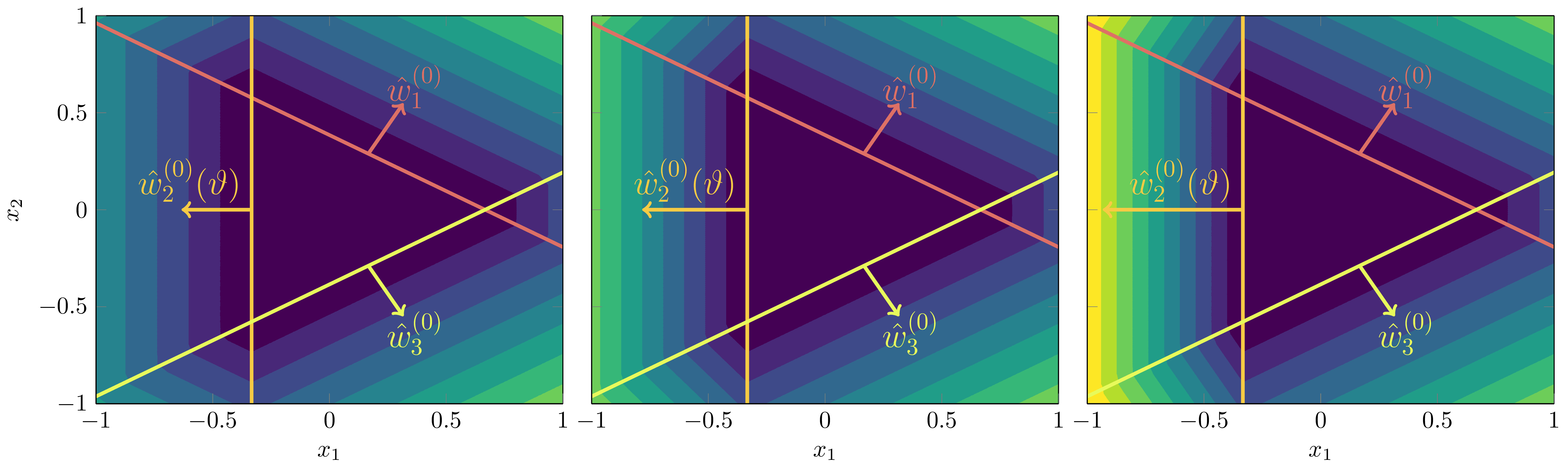
The true weights rotate towards one another by a hyperparameter $\theta =[0,\frac{\pi }{2}]$, so ^[11]

$$w_1^{\left(0\right)}=(\cos \theta ,\sin \theta ),w_2^{\left(0\right)}=(-\cos \theta ,\sin \theta ).$$

As we explained in DSLT3, we can depict the function and its activation boundaries pictorially:

Contour plot of $f_2(x,\theta )$ and its activation boundaries at $\theta =0$ (left), $\theta =\frac{\pi }{4}$ (middle) and $\theta =\frac{\pi }{2}$ (right).

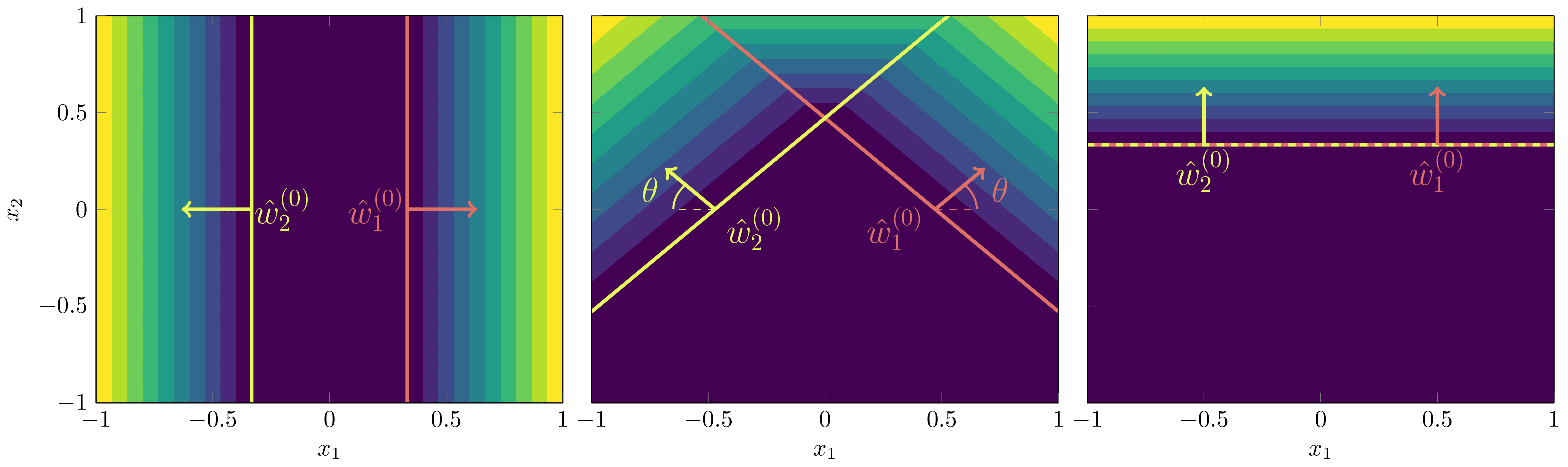
At $\theta =\frac{\pi }{2}$, the truth could be expressed by a network with only one node, $m=1$,

$$f_2(x,\frac{\pi }{2})=ReLU(x_2-\frac{1}{3})+ReLU(x_2-\frac{1}{3})=2ReLU(x_2-\frac{1}{3}).$$

This degeneracy is what we are interested in studying. The WBIC tells us to expect the posterior to prefer the one-degenerate-node configuration since it has less effective parameters. ^[12]

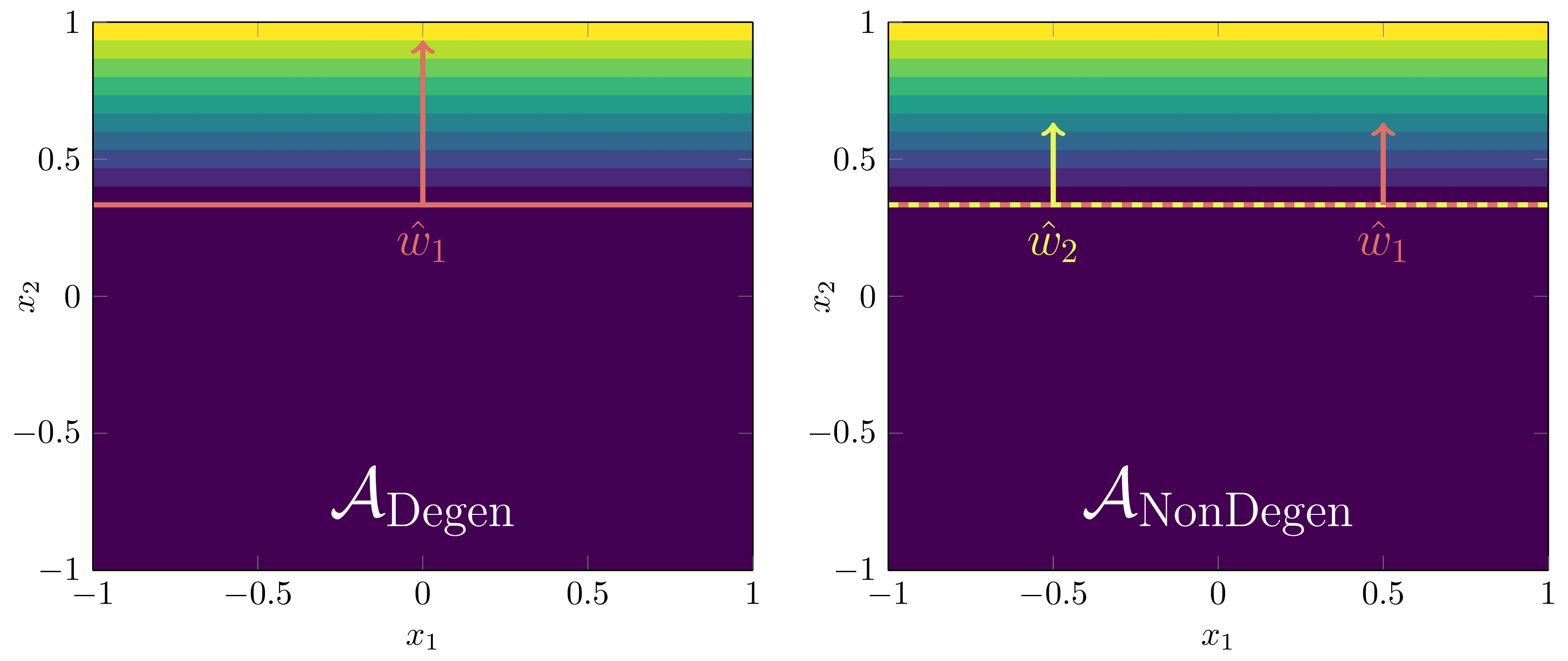
To identify our phases, at $\theta =\frac{\pi }{2}$ there are two possible configurations of the effective model weights that are true parameters:

• Both non-degenerate but share the same activation boundary: Both ${\hat{w}}_1,{\hat{w}}_2\ne 0$ such that ${\hat{w}}_1+{\hat{w}}_2=(0,2)$.

• One degenerate, one non-degenerate: Either ${\hat{w}}_1=(0,0)$ and ${\hat{w}}_2=(0,2)$, or vice versa by permutation symmetry.

To study these configurations we thus define phases based on annuli in the plane centred on the circle of radius $r$ with annuli radius of $\epsilon$,

$$A(r,\epsilon )=\left\{\right({\hat{w}}_{\_,1},{\hat{w}}_{\_,2})\in R^2|r-\epsilon \le \parallel ({\hat{w}}_{\_,1},{\hat{w}}_{\_,2})\parallel \le r+\epsilon \}.$$

Then we define the two phases containing the singularities of interest to be

$$\begin{array}{cc}{A}_{\text{NonDegen}}& =A(1,\epsilon )\times A(1,\epsilon )\\ A_{\text{Degen}}& =\left(A\right(0,\epsilon )\times A(2,\epsilon \left)\right)\cup \left(A\right(2,\epsilon )\times A(0,\epsilon \left)\right)\end{array}.$$

The union is due to the permutation symmetry—which precise node is degenerate doesn’t matter. We will let $A^c=R^2\setminus (A_{\text{NonDegen}}\cup A_{\text{NonDegen}})$.

The phases of interest in the $({\hat{w}}_{i,1},{\hat{w}}_{i,2})$ plane.

There are two questions we seek to answer:

1. At $\theta =\frac{\pi }{2}$, which phase is preferred by the posterior, since both contain true parameters?

2. Is there a first order phase transition at some ${\theta }_c<\frac{\pi }{2}$ where $A_{Degen}$ becomes preferred, even though it doesn’t contain a true parameter?

The weight configuration of each phase at $\frac{\pi }{2}$. Our experiments will test which of these is preferred.

Results

TOP—The posterior samples for each $\theta \in [1,\frac{\pi }{2}]$, where the red dots indicate the true parameters $w_1^{\left(0\right)},w_2^{\left(0\right)}$ being rotated inwards.

BOTTOM—Estimates of the relative frequency of each phase, i.e. $n_A/n$. Do not be confused—these are not free energy curves like in previous figures of the sequence, but they are instead measurements of posterior concentration of each phase at each $\theta$. In other words, the direction is reversed—higher is better!

Notice how there is a first order phase transition at ${\theta }_c=1.26$. Note also that defining the phases according to fixed annuli is not a perfect clustering mechanism, resulting in $A^c$ increasing in relative frequency for middle $\theta$ values. It is merely designed to paint a numerical picture of what we see visually in the changing posterior.

There is also a static facet grid of the key frames if you want a closer inspection.

The results of our experiments show:

1. At $\theta =\frac{\pi }{2}$, the degenerate phase $A_{Degen}$ is preferred.

2. There is a first order phase transition at ${\theta }_c={1.26}^c$ where $A_{Degen}$ becomes preferred, despite not containing a true parameter for $\theta <\frac{\pi }{2}$,

It is unsurprising (yet satisfying) that the degenerate phase $A_{Degen}$ is preferred at $\theta =\frac{\pi }{2}$, in line with what the WBIC tells us to expect. What might be more surprising, though, is that $A_{NonDegen}$ has extremely little posterior density at this $\theta$ value. ^[13]

As we have argued throughout the sequence, the free energy formula suggests that first order phase transitions happen when there is a change in the accuracy-complexity tradeoff such that the posterior newly preferences one phase over the other. Here, the first order phase transition at ${\theta }_c={1.26}^c$ can be understood in these terms with the following graph that depicts how the accuracy of $A_{Degen}$ improves with $\theta$.

The inaccuracy ${min}_{w\in W}{L}_n\left(w\right)$ of each phase $W$ changes with $\theta$. The variations in the inaccuracy are closely correlated to the underlying accuracy of the truth $L_n\left(w^{\left(0\right)}\right)=S_n$, which are random variations since the truth is itself a random variable since it is $f_2(x,\theta )$ + Gaussian noise. Increasing $n$ and averaging over more trials would hopefully smooth out these curves. Nonetheless, it is clear that the phase transition occurs at the approximate point where the inaccuracy of the two phases is equal, thus implying the complexity of $A_{Degen}$ is lower since it has higher posterior density for $\theta >{\theta }_c$.

A Complexity Measure for Non-Analytic ReLU Networks

One last thing to point out here is that since $K\left(w\right)$ is not analytic for ReLU neural networks, the RLCT is not a well defined object. Nonetheless, Watanabe has recently proven in this paper that there is a bound on the free energy,

$$F_n\le n{S}_n+{\lambda }_{ReLU}\log n$$

where complexity ${\lambda }_{ReLU}\in Q_{>0}$ is measured by the number of parameters in the smallest compressed network possible to represent the function, as a kind of ‘pseudo’-RLCT. In our case the the complexity is

$$2{\lambda }_{ReLU}=\{\begin{array}{cc}9& \text{for}0<\theta <\frac{\pi }{2}\\ 5& \text{for}\theta =\frac{\pi }{2}\end{array}$$

since there are five parameters required in the degenerate phase and nine in the non-degenerate phase ^[14]. In this way, Watanabe’s work predicts the results we see. This also shows us how the theory of SLT may be generalisable to the non-analytic setting and still give approximately the same essential insights into singular models.

Phase Transition 2 - Orientation Reversing Symmetry

Defining the Model, Truth, and Phases

This time we are going to consider a model network with $d=3$ nodes,

$$f(x,w)=c+\sum _{i=1}^{3}ReLU(⟨{\hat{w}}_i,x⟩+{\hat{b}}_i),$$

and a realisable true network $f_3(x,\vartheta )$ with $m=3$ nodes,

$$f_3(x,\vartheta )=\sum _{i=1}^{3}ReLU(⟨{\hat{w}}_i^{\left(0\right)},x⟩-\frac{1}{3}),$$

where the weights are defined by an order parameter $\vartheta \in [1,3]$ that scales one gradient,

$$w_1^{\left(0\right)}=(\cos \frac{\pi }{3},\sin \frac{\pi }{3}),w_2^{\left(0\right)}\left(\vartheta \right)=\vartheta (\cos \pi ,\sin \pi ),w_3^{\left(0\right)}=(\cos \frac{5\pi }{3},\sin \frac{5\pi }{3}).$$

The network $f_3(x,\vartheta )$ changes with $\vartheta$ by increasing the gradient of the ${\hat{w}}_2^{\left(0\right)}$ vector.

At $\vartheta =1$, the weights satisfy the weight annihilation property,

$$w_1^{\left(0\right)}+w_2^{\left(0\right)}+w_3^{\left(0\right)}=(0,0),$$

meaning that reversing the orientation of the weights, $w_i^{\left(0\right)}\mapsto -w_i^{\left(0\right)}$ (which is equal to a rotation by $\pi$), will preserve the function as discussed in DSLT3 - Orientation Reversal. We will use the label weight annihilation phase to refer to the configuration of nodes such that the weights all point into the centre region and annihilate one another.^[15] Our key question thus becomes: does the posterior prefers the weight annihilation phase, or the non-weight annihilation phase, at $\vartheta =1$?

Since ${\sum }_{i=1}^3{w}_i^{\left(0\right)}=0$, the orientation reversing symmetry is present, meaning we want to analyse whether the posterior prefers the weight annihilation phase or the non-weight annihilation phase.

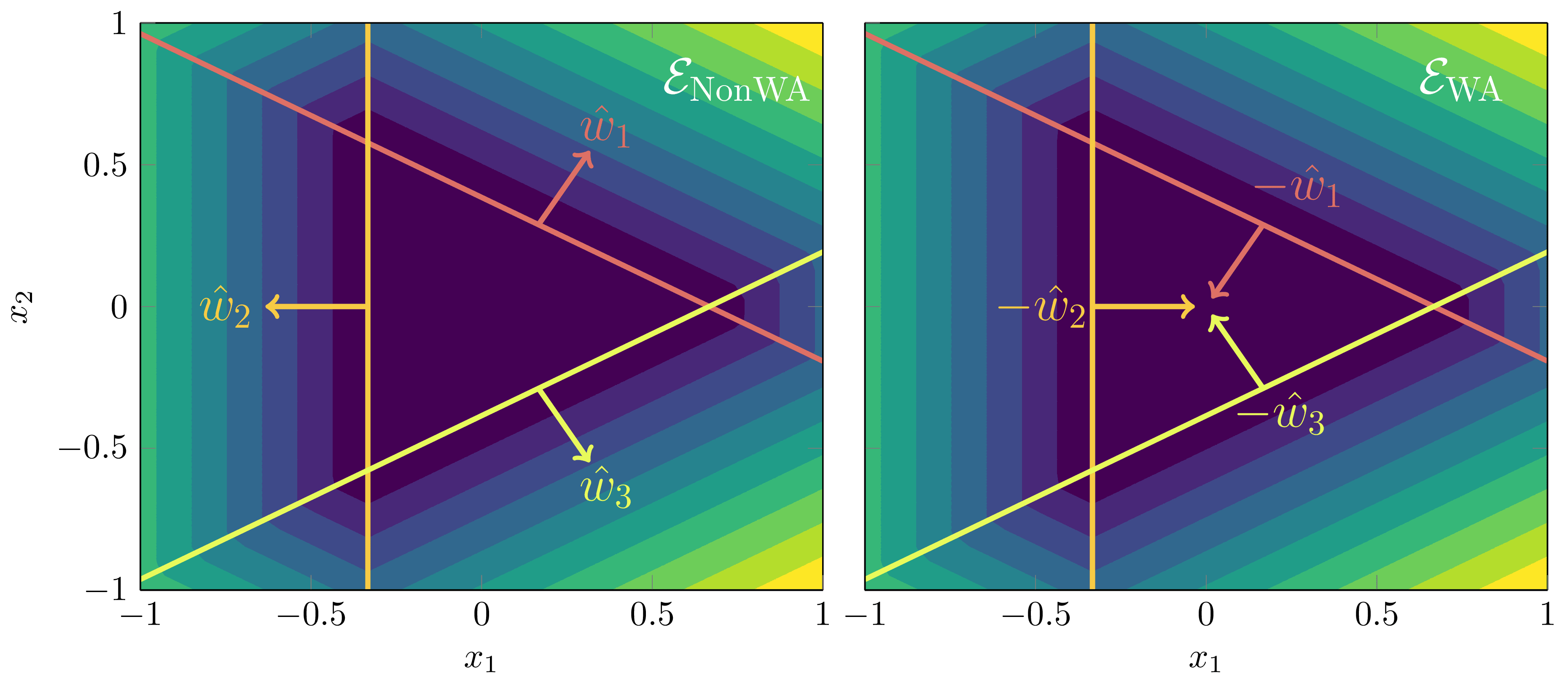
To depict the phases on the $(w_{i,1},w_{i,2})$ plane, let $R\left(\theta \right)=(\cos \theta ,\sin \theta )$, let $B(x,\epsilon )$ be the closed ball of radius epsilon centred at $x\in R^2$, and let $S_3$ denote the permutation group of order 3. Then the two phases of interest are

$$\begin{array}{cc}{E}_{\text{NonWA}}& =\bigcup _{\sigma \in S_3}\prod _{k=0}^{2}B(R(\frac{\pi }{3}+\frac{2\sigma \left(k\right)\pi }{3}),\epsilon )\\ E_{\text{WA}}& =\bigcup _{\sigma \in S_3}\prod _{k=0}^{2}B(R\left(\frac{2\sigma \left(k\right)\pi }{3}\right),\epsilon )\end{array}.$$

Since $w_2^{\left(0\right)}$ is being scaled by $\vartheta$, we will understand the centre of each ball corresponding to $\sigma \left(k\right)=1$ in $E_{\text{NonWA}}$ as being multiplied by the scalar $\vartheta$. (It is easier to state in words that writing down in gory notation).

The phases $E_{\text{NonWA}}$ and $E_{\text{WA}}$ in the $(w_{i,1},w_{i,2})$ plane at $\vartheta =1$. As $\vartheta$ increases, the leftmost ball of $E_{\text{NonWA}}$ will shift leftward.

In this experiment our two questions are:

1. At $\vartheta =1$, which phase is preferred?

2. Is there a first or second order phase transition at some ${\vartheta }_c\in (1,3]$?

Results

Posterior samples for each $\vartheta \in [1,3]$, where the red dots are true parameters $w_1^{\left(0\right)},w_2^{\left(0\right)}\left(\vartheta \right),w_3^{\left(0\right)}$.
Notice how the $E_{\text{WA}}$ phase has less posterior concentration at $\vartheta =1$ despite containing a true parameter. There is a second order destruction transition at ${\vartheta }_c\approx 2$ where $W_{\text{WA}}$ ceases to have any mass since its inaccuracy is too high.

The results of this experiment show that:

1. At $\vartheta =1$ the non-weight annihilation phase $E_{\text{NonWA}}$ is preferred by the posterior.

2. The weight annihilation phase $E_{\text{WA}}$ is never preferred by the posterior, thus there is no first order phase transition. But there is a second order phase transition at ${\vartheta }_c\approx 2$ where $E_{\text{WA}}$ is destroyed.

In [Carroll, $\S$5.4.3], I perform a calculation on an even simpler orientation-reversing example which shows that the relative error of inner cancellation region strongly dictates the preference of the two phases. This relative error can be made smaller by increasing the size of the prior $q\left(x\right)$. That result suggests that the two phases may have the same RLCT, but differing lower order geometry. This is speculative though, and it would be interesting to better understand the RLCT of both phases.

The second order phase transition is unsurprising since we specifically deform the network so that $E_{\text{WA}}$ doesn’t contain a true parameter for $\vartheta \in (1,3]$. At ${\vartheta }_c$, its inaccuracy is too highly penalised and the posterior contains no samples from the region.

References

[Callen] - H. Callen, Thermodynamics and an Introduction to Thermostatistics, 1991

[Gilmore] - R. Gilmore, Catastrophe Theory for Scientists and Engineers, 1981

[Wat18] - S. Watanabe, Mathematical Theory of Bayesian Statistics, 2018

[Carroll] - L. Carroll, Phase Transitions in Neural Networks, 2021

[Wei22] - S. Wei, D. Murfet, et al., Deep learning is singular, and that’s good, 2022

---

1. ^

   At constant atmospheric pressure, that is.

2. ^

   Yes, in any physics or chemistry textbook you will see the Gibbs free energy denotes by $G$. I am writing $F$ to keep it consistent with our later statistical learning discussion.

3. ^

   At this point, this is a slight abuse of the physics notions. Typically the probability distribution is proportional to $e^{-\beta H\left(w\right)}$ where $\beta$ is the inverse temperature. In this case we are going to absorb the $\beta$ into the $H(w;\theta )$ term and not get too caught up in the actual physics—we’re just painting a conceptual picture to apply later on.

4. ^

   Which often correspond to the moments (mean, variance, etc.) of quantities like $H\left(w\right)$.

5. ^

   More precisely, considering the tempered posterior at inverse temperature $\beta >0$, the Hamiltonian has the form

   $$H_n\left(w\right)=n\beta L_n\left(w\right)-\log \phi \left(w\right).$$

   (Since $K_n\left(w\right)=L_n\left(w\right)-S_n$, the constant $S_n$ in $w$ is irrelevant).

6. ^

   Note here that a phase transitions of a dynamical system (i.e. SGD, which we can imagine as a particle moving subject to a potential well) is a slightly more subtle concept. One imagines the loss landscape to be fixed, and the “phase transition” corresponding to the particle moving from one particular phase in $W$ to another. In this sense, there isn’t exactly a phase transition in the general sense, but there is a change in which phase a system finds itself in.

7. ^

   Which altered the posterior geometry, but not that of $K\left(w\right)$ since $p\left(w|D_n\right)\approx e^{-nK\left(w\right)}$ (up to a normalisation factor).

8. ^

   It is a little bit disingenuous to continue to call these phases when $\delta$ is very close to 1, as the singularity $w_1^{\left(0\right)}$ has a non-negligible effect on $W_2$, and vice-versa, meaning the phases lose their individual identities. Alternatively, one defines $W_0$ to centre on $w_0^{\left(0\right)}=0$, and observes how the free energy changes with $\delta$. But, I have kept the two “phases” $W_1$ and $W_2$ in the animation below to illustrate the general idea with minimum fuss.

9. ^

   You might wonder why we still endow the model with the $q_i$ parameters in the first place if we just normalise them out after the fact. We assumed it was more important to let the sampling procedure take place on an earnest neural network model without restricting its parameter space, thus trying to keep it in line with neural networks actually used in practice. But, it is likely that these results would hold otherwise, too.

10. ^

    The astute observer will notice that this is a white lie—the functional equivalence is true as long as each $q_i\ge 0$. However, in our experiments, the true outgoing weights are $q_i=1$, meaning a good sample will only ever have positive weights, i.e. any sample with a negative $q_i^{\left(k\right)}$ will be removed by the outlier validation.

11. ^

    Explicitly, the truth is defined by

    $$f_2(x,\theta )=ReLU\left(\cos \right(\theta )x_1+\sin (\theta )x_2-\frac{1}{3})+ReLU(-\cos (\theta )x_1+\sin (\theta )x_2-\frac{1}{3}),$$
12. ^

    Relatedly, the plot of the KL divergence in Example 3.3 tells us to expect that the degenerate phase may be preferred.

13. ^

    It is worth briefly mentioning the effect of the prior here. The free energy formula tells us that as $n\to \infty$, the effects of the prior on learning become negligible. But of course, we are only ever in the finite $n$ regime, at which point the prior does have effects on the posterior. In our case, since the prior is a Gaussian centred at $w=(0,0)$ with standard deviation $1$, it is reasonable to say that it has some bearing on the degenerate phase being preferred. However, further experiments showed that this behaviour is still retained for a flatter prior with increased standard deviation. The problem, however, is that the Markov chains can become very unstable on these priors, producing posterior samples with very high loss, indicating that the chains aren’t converging to the correct long-term distribution. In the interest of time, I decided not to continue to fine-tune the experiments on non-converging chains for a flatter prior, but it would be interesting to see to what extent the prior does affect these results.

14. ^

    In other words, the degenerate phase requires a truth with five parameters

    $$q_1^{\left(0\right)}ReLU(w_{1,1}^{\left(0\right)}{x}_1+w_{1,2}^{\left(0\right)}{x}_2+b_1^{\left(0\right)})+c,$$

    whereas the non-degenerate phase requires nine,

    $$q_1^{\left(0\right)}ReLU(w_{1,1}^{\left(0\right)}{x}_1+w_{1,2}^{\left(0\right)}{x}_2+b_1^{\left(0\right)})+q_2^{\left(0\right)}ReLU(w_{2,1}^{\left(0\right)}{x}_1+w_{2,2}^{\left(0\right)}{x}_2+b_2^{\left(0\right)})+c.$$
15. ^

    @Leon Lang correctly pointed out that this is slightly weird terminology to use. Instead these should really be referred to as weight-cancellation instead of weight-annihilation, since both initial configurations obey the weight-annihilation property as I defined it, whereas what I am really referring to is the fact that in one configuration all weights are active and cancel in a region. It’s too late to change the terminology throughout, but do keep this in mind.

[Edmund Lau]

Thanks for this sequence and great exposition!

[Leon Lang]

Thanks also for this post! I enjoy reading the sequence and look forward to post 5 on the connections to alignment :)

At some critical value $\theta ={\theta }_c$, we recognise a phase transition as being a discontinuous change in the free energy or one of its derivatives, for example the generalisation error $G_n=E\left[F_{n+1}\right]-E\left[F_n\right]$.

“Discontinuity” might suggest that this happens fast. Yet, e.g. in work on grokking, it actually turns out that these “sudden changes” happen over a majority of the training time (often, the x-axis is on a logarithmic scale). Is this compatible, or would this suggest that phenomena like grokking aren’t related to the phase transitions predicted by SLT?

There is, however, one fundamentally different kind of “phase transition” that we cannot explain easily with SLT: a phase transition of SGD in time, i.e. the number gradient descent steps. The Bayesian framework of SLT does not really allow one to speak of time—the closest quantity is the number of datapoints $n$, but these are not equivalent. We leave this gap as one of the fundamental open questions of relating SLT to current deep learning practice.

As far as I know, modern transformers are often only trained once on each data sample, which should close the gap between SGD time and the number of data samples quite a bit. Do you agree with that perspective?

In general, it seems to me that we’re probably most interested in phase transitions that happen across SGD time or with more data samples, whereas phase transitions related to other hyperparameters (for example, varying the truth as in your examples here) are maybe less crucial. Would you agree with that?

Would you expect that most phase transitions in SGD time or the number of data samples are first-order transitions (as is the case when there is a loss-complexity tradeoff), or can you conceive of second-order phase transitions that might be relevant in that context as well?

Which altered the posterior geometry, but not that of $K\left(w\right)$ since $p\left(w|D_n\right)\approx e^{-nK\left(w\right)}$ (up to a normalisation factor).

I didn’t understand this footnote.

but the node-degeneracy and orientation-reversing symmetries only occur under precise configurations of the truth.

Hhm, I thought that these symmetries are about configurations of the parameter vector, irrespective of whether it is the “true” vector or not.
Are you maybe trying to say the following? The truth determines which parameter vectors are preferred by the free energy, e.g. those close to the truth. For some truths, we will have more symmetries around the truth, and thus lower RLCT for regions preferred by the posterior.

We will use the label weight annihilation phase to refer to the configuration of nodes such that the weights all point into the centre region and annihilate one another.

It seems to me that in the other phase, the weights also annihilate each other, so the “non-weight annihilation phase” is a somewhat weird terminology. Or did I miss something?

The weight annihilation phase $E_{\text{NonWA}}$ is never preferred by the posterior

I think there is a typo and you meant $E_{\text{WA}}$.

[Liam Carroll]

“Discontinuity” might suggest that this happens fast. Yet, e.g. in work on grokking, it actually turns out that these “sudden changes” happen over a majority of the training time (often, the x-axis is on a logarithmic scale). Is this compatible, or would this suggest that phenomena like grokking aren’t related to the phase transitions predicted by SLT?

This is a great question and something that come up at the recent summit. We would definitely say that the model is in two different phases before and after grokking (i.e. when the test error is flat), but it’s an interesting question to consider whats going on over that long period of time where the error is slowly decreasing. I imagine that it is a relatively large model (from an SLT point of view, which means not very large at all from normal ML pov), meaning there would be a plethora of different singularities in the loss landscape. My best guess is that it is undergoing many phase transitions across that entire period, where it is finding regions of lower and lower RLCT but equal accuracy. I expect there to be some work done in the next few months applying SLT to the grokking work.

As far as I know, modern transformers are often only trained once on each data sample, which should close the gap between SGD time and the number of data samples quite a bit. Do you agree with that perspective?

This is a very interesting point. I broadly agree with this and think it is worth thinking more about, and could be a very useful simplifying assumption in considering the connection between SGD and SLT.

In general, it seems to me that we’re probably most interested in phase transitions that happen across SGD time or with more data samples, whereas phase transitions related to other hyperparameters (for example, varying the truth as in your examples here) are maybe less crucial. Would you agree with that?

Broadly speaking, yes. With that said, hyperparameters in the model are probably interesting too (although maybe more from a capabilities standpoint). I think phase transitions in the truth are also probably interesting in the sense of dataset bias, i.e. what changes about a model’s behaviour when we include or exclude certain data? Worth noting here that the Toy Models of Superposition work explicitly deals in phase transitions in the truth, so there’s definitely a lot of value to be had from studying how variations in the truth induce phase transitions, and what these ramifications are in other things we care about.

Would you expect that most phase transitions in SGD time or the number of data samples are first-order transitions (as is the case when there is a loss-complexity tradeoff), or can you conceive of second-order phase transitions that might be relevant in that context as well?

At a first pass, one might say that second-order phase transitions correspond to something like the formation of circuits. I think there are definitely reasons to believe both happen during training.

Which altered the posterior geometry, but not that of $K\left(w\right)$ since $p\left(w|D_n\right)\approx e^{-nK\left(w\right)}$ (up to a normalisation factor).

I didn’t understand this footnote.

I just mean that $K\left(w\right)$ is not affected by $n$ (even though of course $K_n\left(w\right)$ or $L_n\left(w\right)$ is), but the posterior is still affected by $n$. So the phase transition merely concerns the posterior and not the loss landscape.

but the node-degeneracy and orientation-reversing symmetries only occur under precise configurations of the truth.

Hhm, I thought that these symmetries are about configurations of the parameter vector, irrespective of whether it is the “true” vector or not.

My use of the word “symmetry” here is probably a bit confusing and a hangover from my thesis. What I mean is, these two configurations are only in the set of true parameters in this setup when the truth is configured in a particular way. In other words, they are always local minima of $K\left(w\right)$, but not always global minima. (This is what PT1 shows when $1.26\le \theta <\frac{\pi }{2}$). Thanks for pointing this out.

It seems to me that in the other phase, the weights also annihilate each other, so the “non-weight annihilation phase” is a somewhat weird terminology. Or did I miss something?

Huh, I’d never really thought of this, but I now agree it is slightly weird terminology in some sense. I probably should have called them the weight-cancellation and non-weight-cancellation phases as I described in the reply to your DSLT3 comment. My bad. I think its a bit too late to change now, though.

I think there is a typo and you meant $E_{\text{WA}}$.

Thanks! And thanks for reading all of the posts so thoroughly and helping clarify a few sloppy pieces of terminology and notation, I really appreciate it.