Race Along Rashomon Ridge
Produced As Part Of The SERI ML Alignment Theory Scholars Program 2022 Research Sprint Under John Wentworth
Two Deep Neural Networks with wildly different parameters can produce equally good results. Not only can a tweak to parameters leave performance unchanged, but in many cases, two neural networks with completely different weights and biases produce identical outputs for any input.
The motivating question:
Given two optimal models in a neural network’s weight space, is it possible to find a path between them comprised entirely of other optimal models?
In other words, can we find a continuous path of tweaks from the first optimal model to the second without reducing performance at any point in the process?
Ultimately, we hope that the study of equivalently optimal models would lead to advances in interpretability: for example, by producing models that are simultaneously optimal and interpretable.
Introduction
Your friend has invited you to go hiking in the Swiss Alps. Despite extensive planning, you completely failed to clarify which mountain you were supposed to climb. So now you’re both currently standing on different mountaintops Communicating via yodels, your friend requests that you hike over to the mountain he’s already on; after all, he was the one who organised the trip.
How should you reach your friend? A straight line path would certainly work, but it’s such a hassle. Hiking all the way back down and then up another mountain? Madness.
Looking at your map, you notice there’s a long ridge that leaves your mountain at roughly the same height. Does this ridge lead to reach your friend’s mountain and is it possible to follow this ridge to reach your friend?
Similarly, we can envision two optimal models in a neural net’s weight space that share a “ridge” in the loss landscape. There is a natural intuition that we should be able to “walk” between these two points without leaving the ridge. Does this intuition hold up? And what of two neural networks some distance apart in the loss landscape that have both gotten close to the global minima? Can we find a way to walk from one to the other without leaving the ridge?
To begin our investigation into the structure of these “ridges” we viewed these structures as comprising the Rashomon manifold, the subset of the weight space comprised of models that minimize the loss function. In the 2018 paper, Garipov et al. demonstrated that a simple curve is often sufficient to connect two points within the Rashomon manifold.
In our research, we applied the technique of Garipov et al. to path-connect, within a shared weight space, two models that have been trained to be optimal (at an image recognition task with respect to a given dataset). Then, we collected local data along the connecting path. One such local datum is the Hessian of the loss function with respect to the parameters. Its eigendecomposition tells us which directions to travel locally if we want to leave the Rashomon manifold, as well as which directions to travel locally if we want to stay within it. We present a formal description below.
Theory
Consider a neural net.
Let denote the weight parameters of the trained model yielded by the neural net.
Let denote the loss function, a real-valued function on the parameter space that the model has been trained to minimize. Assume the loss function is “nice and smooth″; for example, a neural net that uses skip architecture tends to produce a nice, smooth loss landscape.
We should expect the local minima of a nice loss function to be divided into connected “ridges.” Formally, if the loss function is smooth and moreover a submersion, then every level set is a manifold. In particular, the level set of optimal models is a manifold, whose connected components are the “ridges.” A manifold is a geometric shape that looks locally, but not necessarily globally, like Euclidean space (like for some finite , which is the dimension of the manifold). An example of a manifold is a circle, which locally looks like a one-dimensional line, but not globally. A smooth manifold is a manifold without any kinks or corners. Contrast a circle, which is a smooth 1-dimensional manifold, with a star outline, which is a non-smooth 1-dimensional manifold.
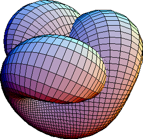
Of course, the manifold comprised of optimal models is going to be a lot more complicated and higher-dimensional. The following example is illustrative of how difficult it is in general to globally visualize manifolds, even if they are nice spaces that are locally Euclidean.
So OK, let’s say for the sake of argument that the set of optimal models is a (locally) nice manifold, even if it’s difficult to visualize. What do we know about its structure?
Empirical work suggests the following pattern. When the class of models is underparametrized (i.e., low-dimensional linear regression, small-scale neural net architecture), there can be many ridges of local minima. This means that the precise choices of the initial parameter vector and of the optimization method (e.g., gradient descent without dropout vs. with dropout) can affect the ridge that the model will fall into during training.
However, when the class of models is sufficiently overparametrized (i.e., large-scale neural net architecture), we suspect they eventually have just one connected ridge of local minima: the ridge of global minima. The dimension of this single ridge is smaller than the dimension of the whole weight space, but still quite high-dimensional. Intuitively, the large number of linearly independent zero-loss directions at a global minimum allow for many opportunities to path-connect to a local minimum while staying within the ridge, making all local minima globally minimal.
There are two ways to think about the ridge of global minima. The first way, common in the literature (see, for example, Semonova et al. and Section 9 here), is to consider the subset of models in the parameter space that achieve sufficiently low loss. This subset is called the Rashomon set:
Let for a positive , where is the global minimum. If is sufficiently small, the Rashomon set becomes a sufficiently sparse subset of the parameter space .
We propose a second way. We consider the Rashomon set as the set of all global minimizers,
.
It is plausible that the level set of global minimizers is a connected smooth submanifold. (This is often true in differential geometry. As long as is a “nice” type of map called a submersion, every level set is a smooth embedded submanifold of the domain .)
We call the submanifold of optimal models the Rashomon manifold, distinct from “Rashomon set’” (to distinguish from the first definition). Note that the first definition is highly related to the second definition. The Rashomon set denoting the first definition,
is a “thickening” of the Rashomon manifold denoting the second definition.
How might this help deep-learning interpretability? By knowing the data of the Rashomon manifold , we can hope to find an element in the intersection for a subset of interpretable models in the total model space. The neural-net model corresponding to this element would be simultaneously interpretable and optimal.
If the subset of interpretable models is also “nice” in the differential-geometric sense (say, also a smooth submanifold of ), then the intersection is also similarly “nice.” This means that we may be able to use tools from differential geometry to probe for an element in this “nice” intersection: an example of a model that is simultaneously interpretable and optimal. These differential-geometric tools include bundles, vector fields, differential forms, parallel transport, and flows.
One potential choice of a subset of interpretable models which is geometrically “nice″ is the submanifold of models which is prunable in a certain way. For example, the submanifold defined by the system of equations , where are the output connections of a given neuron , is comprised of models which can be pruned by removing neuron number . Thus, we may be able to maximally prune a neural net (with respect to the given dataset) by using an algorithm of the following form:
Find in the Rashomon manifold an optimal model that can be pruned in some way.
Prune the neural net in that way.
Repeat Steps 1 and 2 until there are no simultaneously prunable and optimal models anymore.
It is consequently plausible that studying the Rashomon manifold will be crucial for deep-learning interpretability.
How can we study the Rashomon manifold? One way is to take the Hessian of the loss function at a point and find the number of zero eigenvalues: the number of linearly independent zero-loss directions when locally starting from . This number is the dimension of the Rashomon manifold. (See Sagun et al. for an example of this approach.)
To see why this is true, let us investigate what the Hessian is, and why it is important for probing local selection pressures at an optimal model.
The Hessian of a function is defined by the matrix of second derivatives,
.
A three-dimensional example is helpful. Consider the submanifold of cut out by the loss function . The global mimimum of is , and the Rashomon manifold, given by
,
is the -axis.
is the -axis.
is a thickened ellipse cylinder.
the boundary of the ellipse cylinder.
It is hollow, not thickened.
Choose any optimal model on this line, say . Since this point is on the Rashomon manifold, we have ; the gradient vanishes at this point . So, the dominant local effects, the dominant selection pressures, are second-order. At , a small perturbation in the direction of any vector with zero in the -entry will result in an accelerating penalty to the loss function. The acceleration rate is when going along either the positive or the negative -direction. The acceleration rate is when going along either the positive or the negative -direction. These directions correspond to the major and the minor axes of the ellipses you get by looking at level sets for small (while keeping the zero-loss direction’s variable, , to be constant).
And indeed, the ellipse axes’ directions and lengths are precisely captured by the Hessian matrix at ,
.
The eigenvectors and represent the directions of the axes of the local selection effects’ parabola, and their corresponding eigenvalues and represent the magnitudes of the selection pressures in these axes’ directions. The zero eigenvector is the sole zero-loss direction at point : the sole direction starting from that remains contained in the Rashomon manifold. This is because the Rashomon manifold of is one-dimensional (indeed, it is the -axis).
The Hessian of a higher-dimensional loss function essentially behaves in the same way. The eigenvectors with positive eigenvalue serve as (hyper)ellipsoid axes that span the nonzero-loss directions. When moving in these directions, one experiences an accelerating penalty to the loss function.
The eigenvectors with zero eigenvalue span the zero-loss directions. When moving in these directions, one remains in the Rashomon set.
And since every point of the Rashomon manifold is a global minimizer, and therefore also a local minimizer, negative eigenvalues do not occur. In math terminology, the Hessian matrix is positive-semidefinite at every local minimizer.
The Hessian at a given point on the Rashomon manifold is an example of local data. The dimension of the Rashomon manifold is an example of global data. Generally, we can hope to compute sufficiently many local and/or global data of the Rashomon manifold, enough to (1) prove or disprove the nonemptiness of , and if the former is true, (2) construct one such point in . This can potentially be done via tools from differential geometry, or from the more broadly applicable tools of topology. Successfully doing so would yield a simultaneously optimal and interpretable model for the given dataset.
Procedure
As mentioned above, we first reproduced the results of this paper on connectivity between optima, using a smaller architecture of PreResNet20 (~270k params) .
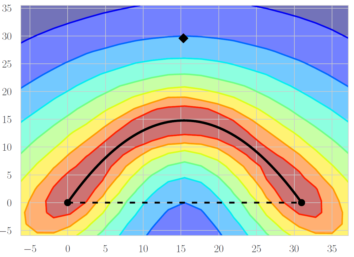
This is a Bézier curve connecting 2 separately trained models along the same ridge in the loss landscape. The dashed line is a straight line path between the 2 weight vectors. The contour plot was made by calculating losses in a grid pattern.
For different points along this curve we have calculated.
A Jacobian of outputs with respect to inputs. Can be used for linear probes of functionality and may be able to identify how the network changes across the ridge.
A Jacobian of loss with respect to params (as expected was close to 0 norm)
The norms of the Vector Hessian Products in the straight line path direction (-axis on the graph), the detour direction (-axis on graph), and the tangent line to the curve of .
Future Pathways
Unfortunately, the nature of a sprint means we couldn’t dedicate as much time to this as we would have liked. To investigate the Hessian within the Rashomon Set more closely we need significantly more computing power or a perhaps a more careful analytic approach.
We are also very keen to explore the structure of the Rashomon set. Specifically we believe much can be gleaned from exploring symmetries in the set.
Take more Hessian vector products of models moving in the direction of the vector. Combine these values in some way to get a better estimate. The Hessian vector product on the tangent direction to the constant loss curve was smaller, but not zero like we expected and this may be due to noise.
Use linear probes on the Jacobians of outputs with respect to inputs to identify functional similarities and differences between the models on the curve. The paper by Garipov et. al. showed that an ensemble of these models performs better than an individual one, which implies that some functional differences exist and the ridge is not simply due to irrelevant parameters.
Jacobian of outputs with respect to parameters. Due to cuda running out of the 6gb gpu memory on my laptop.
Using PyHessian to get top eigenvalues, trace and eigenvalue density of the Hessian of loss with respect to params. Getting a memory leak and infinite loop of params self referencing their gradients. This worked once in the colab notebook, so I have a suspicion it is a windows version bug. This is the graph that generated.
Using the density graph at different points we should be able to determine if the number of dimensions on the ridge remains constant.
Another possibility is using the fast ensembling method of using a cyclic learning rate schedule to move along the ridge by leaving it and converging back to it in a different place. This should get models in many directions on the ridge instead of following a single curve.
Various takes on this research direction, from someone who hasn’t thought about it very much:
I think that the answer here is definitely no, without further assumptions. For example, consider the case where you have a model with two ReLU neurons that, for optimal models, are doing different things; the model where you swap the two neurons is equally performant, but there’s no continuous path between these models.
More concretely, imagine that we want to learn (y1, y2) = (ReLU(x1), ReLU(x2)) with a model of the form
where a through h are parameters. In Pytorch we’d write this as
W2 @ relu(W1 @ x), for W1 and W2 of shape [2, 2].We can model the true function perfectly by either using the first neuron for x1 and the second for x2 or vice versa, but there’s no continuous path between them.
(As a simpler example, consider the task of choosing parameters a and b such that a*b = 1. There’s no continuous path from the (1, 1) solution to the (-1, −1) solution.)
Plausibly you could choose some further assumptions that make this true. You gesture at this a little:
But IMO a whole lot of the work here is going to be choosing a definition of “sufficiently overparameterized” such that the theorem isn’t easily counterexampled.
And from a relevance-to-alignment standpoint, I think it’s pretty likely that if you succeed at finding a definition of “sufficiently overparameterized” such that this is true, that definition will require that the model is sufficiently “larger” than the task it’s modeling that it will seem implausible that the theorem will apply in the real world (given that I expect the real world to be “larger” than AGIs we train, and so don’t expect AGIs to be wildly overparameterized).
Another way of phrasing my core objection: the original question without further assumptions seems equivalent to “given two global minima of a function, is there a path between them entirely comprised of global minima”, which is obviously false.
Hey Buck, love the line of thinking.
We definitely aren’t trying to say “any two ridges can be connected for any loss landscape” but rather that the ridges for overparameterised networks are connected.
TL;DR: I agree that the answer to the question above definitely isn’t always yes, because of your counterexample, but I think that moving forward on a similar research direction might be useful anyways.
One can imagine partitioning the parameter space into sets that arrive at basins where each model in the basin has the same, locally optimal performance, this is like a Rashomon set (relaxing the requirement from global minima so that we get a partition of the space). The models which can compress the training data (and thus have free parameters) are generally more likely to be found by random selection and search, because the free parameters means that the dimensionality of this set is higher, and hence exponentially more likely.
Thus, we can move within these high-dimensional regions of locally optimal loss, which could allow us to find more interpretable (or maybe more desirable along another axis), which is the stated motivation in the article:
This seems super relevant to alignment! The default path to AGI right now to me seems like something like a LLM world model hooked up to some RL to make it more agenty, and I expect this kind of theory applied to LLMs, because of the large number of parameters. I’m hoping that this theory gets us better predictions on which Rashomon sets are found (this would look like a selection theorem), and the ability to move within a Rashomon set towards parameters that are better. Such a selection theorem seems likely because of the dimensionality argument above.
Edit: Adding a link to “Git Re-Basin: Merging Models modulo Permutation Symmetries,” a relevant paper that has recently been posted on arXiv.
Thank you so much, Thomas and Buck, for reading the post and for your insightful comments!
It is indeed true that some functions have two global minimizers that are not path-connected. Empirically, very overparametrized models which are trained on “non-artificial” datasets (“datasets from nature”?) seem to have a connected Rashomon manifold. It would definitely be helpful to know theoretically why this tends to happen, and when this wouldn’t happen.
One heuristic argument for why two disconnected global minimizers might only happen in “artificial” datasets might go something like this. Given two quantities, one is larger than the other, unless there is a symmetry-based reason why they are actually secretly the same quantity. Under this heuristic, a non-overparametrized model’s loss landscape has a global minimum achieved by precisely one point, and potentially some suboptimal local minima as well. But overparametrizing the model makes the suboptimal local minima not local minima anymore (by making them saddle points?) while the single global minimizer is “stretched out” to a whole submanifold. This “stretching out” is the symmetry; all optimal models on this submanifold are secretly the same.
One situation where this heuristic fails is if there are other types of symmetry, like rotation. Then, applying this move to a global minimizer could get you other global minimizers which are not connected to each other. In this case, “modding out by the symmetry” is not decreasing the dimension, but taking the quotient by the symmetry group which gives you a quotient space of the same dimension. I’m guessing these types of situations are more common in “artificial” datasets which have not modded out all the obvious symmetries yet.
In your example, I think even adding just one more node, h3, to the hidden layer would suffice to connect the two solutions. One node per dimension of input suffices to learn the function, but it’s also possible for two nodes to share the task between them, where the share of the task they are picking up can vary continuously from 0 to 1. So just have h3 take over x2 from h2, then h2 takes over x1 from h1, and then h1 takes over x2 from h3.
Yeah, but you have the same problem if you were using all three of the nodes in the hidden layer.
Actual trained neural networks are known to have redundant parameters, as demonstrated by the fact that we can prune them so much.
Have you seen this paper? They find that “SGD solutions are connected via a piecewise linear path, and the increase in loss along this path vanishes as the number of neurons grows large.”
Interesting stuff. Prunability might not be great for interpretability—you might want something more like sparsity, or alignment of the neuron basis with specified human-interpretable classifications of the data.
Thanks so much, Charlie, for reading the post and for your comment! I really appreciate it.
I think both ways to prune neurons and ways to make the neural net more sparse are very promising steps towards constructing a simultaneously optimal and interpretable model.
I completely agree that alignment of the neuron basis with human-interpretable classifications of the data would really help interpretability. But if only a subset of the neuron basis are aligned with human-interpretability, and the complement comprises a very large subset of abstractions (which, necessarily, people would not be able to learn to interpret), then we haven’t made the model interpretable.
Suppose 100% is the level of interpretability we need for guaranteed alignment (which I am convinced of, because even 1% uninterpretability can screw you over). Then low-dimensionality seems like a necessary, but not sufficient condition for intepretability. It is possible, but not always true, that each of a small number of abstractions will either already familiar to people or can be learned by people in a reasonable amount of time.
“ridge to” → “ridge”,
”possible” to “Is it possible”.
“that eventually have” → “they eventually have”,
“path-connect towards” - > “path connect to”.
Considering getting a linter for your browser, like https://languagetool.org, to avoid these sorts of errors in future.
This is clever, and also seems like the core idea of the post. You should put this info at the start.
This is a nice write-up, thanks for sharing it.
It seems like it’s possible to design models that always have this property. For any model M, consider two copies of it, M’ and M″. We can construct a third model N that is composed of M’ and M″ plus a single extra weight p (with 0 ⇐ p ⇐ 1). Define N to have output by running the input on M’ and M″ and choose the result of M’ with probability p and otherwise the result of M″. Any N achieves minimal loss if and only if it’s one of the following cases:
M’ and M″ are both individually optimal and 0 < p < 1,
M’ is optimal and p = 1 (M″ arbitrary), or
M″ is optimal and p = 0 (M’ arbitrary).
Then to get a path between any optimal weights, we just move to p = 0, modify M″ as desired, then move to p=1 and modify M’ as desired, then set p as desired. I think there’s a few more details than this; it probably depends upon some properties of the loss function, for example, that it doesn’t depend upon the weights of M only the output.
Unfortunately this doesn’t help us at all in this case! I don’t think it’s any more interpretable than M alone. So maybe this example isn’t useful.
Also, don’t submersions never have (local or global) minima? Their derivative is surjective so can never be zero. Pretty nice-looking loss functions end up not having manifolds for their minimizing sets, like x^2y^2. I have a hard time reasoning about whether this is typical or atypical though. I don’t even have an intuition for why the global minimizer isn’t (nearly always) just a point. Any explanation for that observation in practice?
I agree, and believe that the post should not have mentioned submersions.
I agree that the typical function has only one (or zero) global minimizer. But in the case of overparametrized smooth Neural Networks it can be typical that zero loss can be achieved. Then the set of weights that lead to zero loss is typically a manifold, and not a single point. Some intuition: Consider linear regression with more parameters than data. Then the typical outcome is a perfect match of the data, and the possible solution space is a (possibly high-dimensional) linear manifold. We should expect the same to be true for smooth nonlinear neural networks, because locally they are linear.
Note that the above does not hold when we e.g. add a l2-Penalty for the weights: Then I expect there to be a single global minimizer in the typical case.
Thank you so much for this suggestion, tgb and harfe! I completely agree, and this was entirely my error in our team’s collaborative post. The fact that the level sets of submersions are nice submanifolds has nothing to do with the level set of global minimizers.
I think we will be revising this post in the near future reflecting this and other errors.
(For example, the Hessian tells you what the directions whose second-order penalty to loss are zero, but it doesn’t necessarily tell you about higher-order penalties to loss, which is something I forgot to mention. A direction that looks like zero-loss when looking at the Hessian may not actually be not actually be zero-loss if it applies, say, a fourth-order penalty to the loss. This could only be probed by a matrix of fourth derivatives. But I think a heuristic argument suggests that a zero-eigenvalue direction of the Hessian should almost always be an actual zero-loss direction. Let me know if you buy this!)
Do you have any intuition for why we should expect Winterpretable to be “nice”? I’m not super familiar with differential geometry but I don’t really see why this should be the case..