Decoherence

Previously in series: Feynman Paths

To understand the quantum process called “decoherence”, we first need to look at how the special case of quantum independence can be destroyed—how the evolution of a quantum system can produce entanglement where there was formerly independence.

Quantum independence, as you’ll recall, is a special case of amplitude distributions that approximately factorize—amplitude distributions that can be treated as a product of sub-distributions over subspaces.

Reluctant tourists visiting quantum universes think as if the absence of a rectangular plaid pattern is some kind of special ghostly link between particles. Hence the unfortunate term, “quantum entanglement”.

The evolution of a quantum system can produce entanglement where there was formerly independence—turn a rectangular plaid pattern into something else. Quantum independence, being a special case, is easily lost.

Let’s pretend for a moment that we’re looking at a classical system, which will make it easier to see what kind of physical process leads to entanglement.

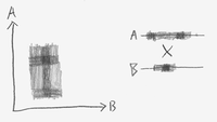
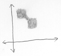
At right is a system in which a positively charged light thingy is on a track, far above a negatively charged heavy thingy on a track.

At the beginning, the two thingies are far enough apart that they’re not significantly interacting.

But then we lower the top track, bringing the two thingies into the range where they can easily attract each other. (Opposite charges attract.)

So the light thingy on top rolls toward the heavy thingy on the bottom. (And the heavy thingy on the bottom rolls a little toward the top thingy, just like an apple attracts the Earth as it falls.)

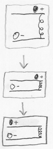
Now switch to the Feynman path integral view. That is, imagine the evolution of a quantum system as a sum over all the paths through configuration space the initial conditions could take.

Suppose the bottom heavy thingy and the top thingy started out in a state of quantum independence, so that we can view the amplitude distribution over the whole system as the product of a “bottom thingy distribution” and a “top thingy distribution”.

The bottom thingy distribution starts with bulges in three places—which, in the Feynman path view, we might think of as three possible starting configurations from which amplitude will flow.

When we lower the top track, the light thingy on top is attracted toward the heavy bottom thingy -

- except that the bottom thingy has a sub-distribution with three bulges in three different positions.

So the end result is a joint distribution in which there are three bulges in the amplitude distribution over joint configuration space, corresponding to three different joint positions of the top thingy and bottom thingy.

I’ve been trying very carefully to avoid saying things like “The bottom thingy is in three places at once” or “in each possibility, the top thingy is attracted to wherever the bottom thingy is”.

Still, you’re probably going to visualize it that way, whether I say it or not. To be honest, that’s how I drew the diagram—I visualized three possibilities and three resulting outcomes. Well, that’s just how a human brain tends to visualize a Feynman path integral.

But this doesn’t mean there are actually three possible ways the universe could be, etc. That’s just a trick for visualizing the path integral. All the amplitude flows actually happen, they are not possibilities.

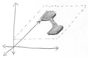
Now imagine that, in the starting state, the bottom thingy has an amplitude-factor that is smeared out over the whole bottom track; and the top thingy has an amplitude-factor in one place. Then the joint distribution over “top thingy, bottom thingy” would start out looking like the plaid pattern at left, and develop into the non-plaid pattern at right:

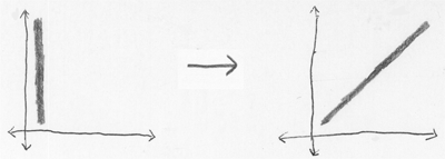
Here the horizontal coordinate corresponds to the top thingy, and the vertical coordinate corresponds to the bottom thingy. So we start with the top thingy localized and the bottom thingy spread out, and then the system develops into a joint distribution where the top thingy and the bottom thingy are in the same place, but their mutual position is spread out. Very loosely speaking.

So an initially factorizable distribution, evolved into an “entangled system”—a joint amplitude distribution that is not viewable as a product of distinct factors over subspaces.

(Important side note: You’ll note that, in the diagram above, system evolution obeyed the second law of thermodynamics, aka Liouville’s Theorem. Quantum evolution conserved the “size of the cloud”, the volume of amplitude, the total amount of grey area in the diagram.

If instead we’d started out with a big light-gray square—meaning that both particles had amplitude-factors widely spread—then the second law of thermodynamics would prohibit the combined system from developing into a tight dark-gray diagonal line.

A system has to start in a low-entropy state to develop into a state of quantum entanglement, as opposed to just a diffuse cloud of amplitude.

Mutual information is also negentropy, remember. Quantum amplitudes aren’t information per se, but the rule is analogous: Amplitude must be highly concentrated to look like a neatly entangled diagonal line, instead of just a big diffuse cloud. If you imagine amplitude distributions as having a “quantum entropy”, then an entangled system has low quantum entropy.)

Okay, so now we’re ready to discuss decoherence.

The system at left is highly entangled—it’s got a joint distribution that looks something like, “There’s two particles, and either they’re both over here, or they’re both over there.”

Yes, I phrased this as if there were two separate possibilities, rather than a single physically real amplitude distribution. Seriously, there’s no good way to use a human brain to talk about quantum physics in English.

But if you can just remember the general rule that saying “possibility” is shorthand for “physically real blob within the amplitude distribution”, then I can describe amplitude distributions a lot faster by using the language of uncertainty. Just remember that it is language. “Either the particle is over here, or it’s over there” means a physically real amplitude distribution with blobs in both places, not that the particle is in one of those places but we don’t know which.

Anyway. Dealing with highly entangled systems is often annoying—for human physicists, not for reality, of course. It’s not just that you’ve got to calculate all the possible outcomes of the different possible starting conditions. (I.e., add up a lot of physically real amplitude flows in a Feynman path integral.) The possible outcomes may interfere with each other. (Which actual possible outcomes would never do, but different blobs in an amplitude distribution do.) Like, maybe the two particles that are both over here, or both over there, meet twenty other particles and do a little dance, and at the conclusion of the path integral, many of the final configurations have received amplitude flows from both initial blobs.

But that kind of extra-annoying entanglement only happens when the blobs in the initial system are close enough that their evolutionary paths can slop over into each other. Like, if the particles were either both here, or both there, but here and there were two light-years apart, then any system evolution taking less than a year, couldn’t have the different possible outcomes overlapping.

Okay, so let’s talk about three particles now.

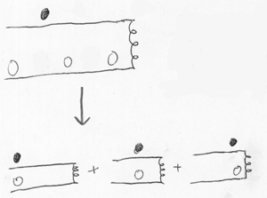
This diagram shows a blob of amplitude that factors into the product of a 2D subspace and a 1D subspace. That is, two entangled particles and one independent particle.

The vertical dimension is the one independent particle, the length and breadth are the two entangled particles.

The independent particle is in one definite place—the cloud of amplitude is vertically narrow. The two entangled particles are either both here, or both there. (Again I’m using that wrong language of uncertainty, words like “definite” and “either”, but you see what I mean.)

Now imagine that the third independent particle interacts with the two entangled particles in a sensitive way. Maybe the third particle is balanced on the top of a hill; and the two entangled particles pass nearby, and attract it magnetically; and the third particle falls off the top of the hill and rolls to the bottom, in that particular direction.

Afterward, the new amplitude distribution might look like this. The third particle is now entangled with the other two particles. And the amplitude distribution as a whole consists of two more widely separated blobs.

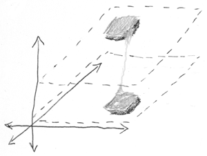
Loosely speaking, in the case where the two entangled particles were over here, the third particle went this way, and in the case where the two entangled particles were over there, the third particle went that way.

So now the final amplitude distribution is fully entangled—it doesn’t factor into subspaces at all.

But the two blobs are more widely separated in the configuration space. Before, each blob of amplitude had two particles in different positions; now each blob of amplitude has three particles in different positions.

Indeed, if the third particle interacted in an especially sensitive way, like being tipped off a hill and sliding down, the new separation could be much larger than the old one.

Actually, it isn’t necessary for a particle to get tipped off a hill. It also works if you’ve got twenty particles interacting with the first two, and ending up entangled with them. Then the new amplitude distribution has got two blobs, each with twenty-two particles in different places. The distance between the two blobs in the joint configuration space is much greater.

And the greater the distance between blobs, the less likely it is that their amplitude flows will intersect each other and interfere with each other.

That’s decoherence. Decoherence is the third key to recovering the classical hallucination, because it makes the blobs behave independently; it lets you treat the whole amplitude distribution as a sum of separated non-interfering blobs.

Indeed, once the blobs have separated, the pattern within a single blob may look a lot more plaid and rectangular—I tried to show that in the diagram above as well.

Thus, the big headache in quantum computing is preventing decoherence. Quantum computing relies on the amplitude distributions staying close enough together in configuration space to interfere with each other. And the environment contains a zillion particles just begging to accidentally interact with your fragile qubits, teasing apart the pieces of your painstakingly sculpted amplitude distribution.

And you can’t just magically make the pieces of the scattered amplitude distribution jump back together—these are blobs in the joint configuration, remember. You’d have to put the environmental particles in the same places, too.

(Sounds pretty irreversible, doesn’t it? Like trying to unscramble an egg? Well, that’s a very good analogy, in fact.

This is why I emphasized earlier that entanglement happens starting from a condition of low entropy. Decoherence is irreversible because it is an essentially thermodynamic process.

It is a fundamental principle of the universe—as far as we can tell—that if you “run the film backward” all the fundamental laws are still obeyed. If you take a movie of an egg falling onto the floor and smashing, and then play the film backward and see a smashed egg leaping off the floor and into a neat shell, you will not see the known laws of physics violated in any particular. All the molecules will just happen to bump into each other in just the right way to make the egg leap off the floor and reassemble. It’s not impossible, just unbelievably improbable.

Likewise with a smashed amplitude distribution suddenly assembling many distantly scattered blobs into mutual coherence—it’s not impossible, just extremely improbable that many distant starting positions would end up sending amplitude flows to nearby final locations. You are far more likely to see the reverse.

Actually, in addition to running the film backward, you’ve got to turn all the positive charges to negative, and reverse left and right (or some other single dimension—essentially you have to turn the universe into its mirror image).

This is known as CPT symmetry, for Charge, Parity, and Time.

CPT symmetry appears to be a really, really, really deep principle of the universe. Trying to violate CPT symmetry doesn’t sound quite as awful to a modern physicist as trying to throw a baseball so hard it travels faster than light. But it’s almost that awful. I’m told that General Relativity Quantum Field Theory requires CPT symmetry, for one thing.

So the fact that decoherence looks like a one-way process, but is only thermodynamically irreversible rather than fundamentally asymmetrical, is a very important point. It means quantum physics obeys CPT symmetry.

It is a universal rule in physics—according to our best current knowledge—that every apparently irreversible process is a special case of the second law of thermodynamics, not the result of time-asymmetric fundamental laws.)

To sum up:

Decoherence is a thermodynamic process of ever-increasing quantum entanglement, which, through an amazing sleight of hand, masquerades as increasing quantum independence: Decoherent blobs don’t interfere with each other, and within a single blob but not the total distribution, the blob is more factorizable into subspaces.

Thus, decoherence is the third key to recovering the classical hallucination. Decoherence lets a human physicist think about one blob at a time, without worrying about how blobs interfere with each other; and the blobs themselves, considered as isolated individuals, are less internally entangled, hence easier to understand. This is a fine thing if you want to pretend the universe is classical, but not so good if you want to factor a million-digit number before the Sun burns out.

Part of The Quantum Physics Sequence

Next post: “The So-Called Heisenberg Uncertainty Principle”

Previous post: “Three Dialogues on Identity”