The central limit theorem in terms of convolutions

[Maxwell Peterson]

There are multiple versions of the central limit theorem. One common version says that, as $n\to \infty$, the mean of means looks like a Gaussian distribution. People in industry sometimes ignore the “goes to infinity” part, and assume that if $n$ is large, that’s good enough. But is that true? When is it safe to assume that your means have converged? I heard of a case recently where the mean of means was assumed to have converged, hadn’t, and the application it was a part of suffered accuracy problems for months without anyone knowing. This sequence will explore: under what conditions does the central limit theorem “fail” like this?

The central limit theorem is about convolutions

There are multiple versions of the central limit theorem. They’re all a version of the statement:

If you have a bunch of distributions $f_i$ (say, $n$ of them), and you convolve them all together into a distribution $F^{\ast }:=f_1\ast f_2\ast f_3...\ast f_n$, then the larger $n$ is, the more $F^{\ast }$ will resemble a Gaussian distribution.

The simplest version of the central limit theorem requires that the distributions $f_i$ must be 1) independent and 2) identically distributed. In this sequence, I’m gonna assume #1 is true. We’ll find that while condition #2 is nice to have, even without it, distributions can converge to a Gaussian under convolution.

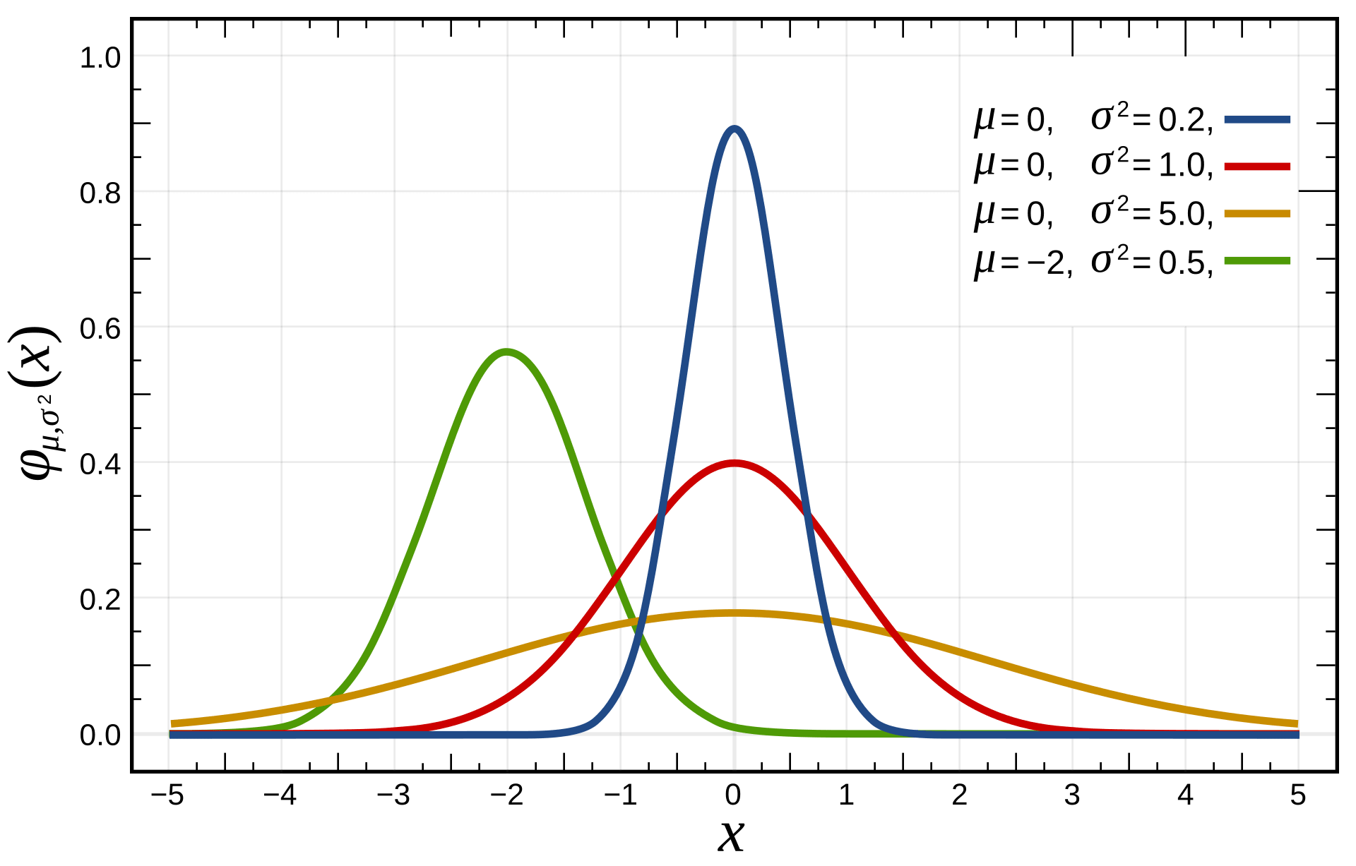
A Gaussian distribution is the same thing as a Normal distribution. Some examples of Gaussian distributions:

Wikipedia

Wait—this doesn’t sound like the central limit theorem I know

Most statements of the central limit theorem, including Wikipedia’s, talk in terms of the sums of random variables (and their density functions and expected values). But this is the same thing as our convolution-of-distributions, because the density function of the sum of two random variables X, Y is the convolution of the density functions of X and Y. Looking at the central limit theorem in terms of convolutions will make it easier to see some things. It’s also useful if your version of probability doesn’t have the concept of a random variable, like probability theory as extended logic*.

Another statement of the central limit theorem, from Jaynes:

The central limit theorem tells us what is essentially a simple combinatorial fact, that out of all conceivable error vectors $e_1,...,e_n$ that could be generated, the overwhelming majority have about the same degree of cancellation.

Hopefully this is enough to convince you that the central limit theorem need not be stated in terms of random variables or samples from a population.

(Also: the central limit theorems are sometimes talked about in terms of means only. They do say things about means, but they also say very much about distributions. I’ll talk about both.)

*: first three chapters here.

Convolutions

The central limit theorem is a statement about the result of a sequence of convolutions. So to understand the central limit theorem, it’s really important to know what convolutions are and to develop a good intuition for them.

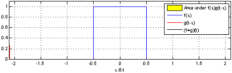
Take two functions, $f$ and $g$. Reverse $g$ on the y-axis, then slide it and $f$ along each other, taking the product of each pair of numbers as you slide. The result is the convolution of $f$and $g$. Here’s a picture - $f$ is blue, $g$ is red, and the convolution $f\ast g$ is black:

Wikipedia

Another one, with a different function $f$:

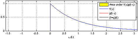
You can write this as $f\ast g={\int }_{-\infty }^{\infty }f\left(x\right)g(x-y)dy$.

The first two sections on this page give a nice explanation of convolutions in terms of dropping a ball twice. This page lets you choose two functions to convolve visually, and I highly recommend it for getting a feel for the operation.

Convolution has nice properties

Convolution is associative and commutative—if you want to convolve multiple functions together, it doesn’t matter what order you do it in. (Also, nothing I’ve said in this section requires $f$ and $g$ to be probability distributions—they can be any two functions.)

You can get the mean of a convolution without actually doing the convolutions. If the first moments of $f$ and g are $F_1$ and $G_1$ (for probability distributions, the first moment is the mean), then the first moment of $f\ast g$ is $F_1+G_1$. There is a hint here about why people often talk about means when they talk about the central limit theorem—being able to get the mean of the convolution by just adding the means of the underlying distributions together is really nice.

You can get the second moment without actually convolving, too. (the second moment is closely related to the variance: if the mean is 0, the second moment and the variance are the same). For $f$ and $g$ with second moments $F_2$, $G_2$, the second moment of $f\ast g$ is $F_2+2F_1{G}_1+G_2$. And so on for higher moments, for as long as $f$ and $g$ actually have those higher moments themselves.

If $F\left\{f\right\}$ and $F\left\{g\right\}$ are the Fourier transforms of $f$ and $g$, then $F\{f\ast g\}=F\left\{f\right\}F\left\{g\right\}$. This is very useful for computing convolutions numerically: evaluating ${\int }_{-\infty }^{\infty }f\left(x\right)g(x-y)dy$ naively would require doing an integral for every single $x$ value you were interested in. That’s expensive, time-wise. Much easier to compute $F\left\{f\right\}$ and $F\left\{g\right\}$ and then just multiply them (multiplication is cheap). After that, applying the inverse Fourier transform gives $f\ast g$. This is how convolution is computed in popular numerical programming languages.

If $f$ sums to 1 and $g$ sums to 1, then $f\ast g$ sums to 1. So if $f$ and $g$ are probability distributions, so is $f\ast g$.

In the next post, I’ll look at what happens when you convolve a bunch of different distributions together, and explore how much of what happens depends on the form of those distributions.

---

Post script: not neural networks

You may have heard of convolutional neural networks from all their success in image processing. I think they involve the same convolution I’m talking about here, but in much higher dimensions. I’ll only be talking about convolutions of one-dimensional functions in this sequence. Some (or a lot?) of the stuff I’ll say about the central limit theorem probably applies in higher dimensions too, but I’m not sure what changes as the dimension increases. So, this sequence is not about the neural networks.

[gjm]

Nitpick: I think you’re mixing up the variance and the second moment. The variance equals the second moment when the mean is zero, but not in general. The theorem with $F_2+2F_1{G}_1+G_2$ in it is about second moments, not variances. The corresponding theorem for variances just says that the variance of the sum equals the sum of the variances (when the distributions are independent, if you’re talking about probability distributions rather than arbitrary functions, which if you use the word “variance” you ought to be). If you use central moments (in which case the second moment is the same thing as the variance) then I guess this theorem is true, but in a rather silly way because then $F_1$ and $G_1$ are necessarily zero.

[Maxwell Peterson]

I definitely was thinking they were literally the same in every case! I corrected that part and learned something. Thanks!

[DaemonicSigil]

Thanks for the interesting post. Looking forward to seeing where this series is going. Mostly for my own understanding, I’m going to mess around with fourier transforms and convolutions in this comment.

Proof that the fourier transform of the convolution of 2 functions is the product of their fourier transforms:

$$F[f\star g]=\int dt{e}^{-i\omega t}\int d\tau f\left(\tau \right)g(t-\tau )$$

$$=\int d\tau f\left(\tau \right)e^{-i\omega \tau }\int dt{e}^{-i\omega (t-\tau )}g(t-\tau )$$

Let $u=t-\tau$. Then, holding $\tau$ constant, $du=dt$. So:

$$F[f\star g]=\int d\tau f\left(\tau \right)e^{-i\omega \tau }\int du{e}^{-i\omega u}g\left(u\right)=F\left[f\right]F\left[g\right]$$

Fourier transform of a general Gaussian distribution, $G\left(t\right)=e^{-(\frac{t-\mu }{\sigma }{)}^2}$:

$$F\left[G\right]\left(\omega \right)=\int dt{e}^{-(\frac{t-\mu }{\sigma }{)}^2}{e}^{-i\omega t}$$

Let $u=t-\mu$.

$$=\int du{e}^{-(\frac{u}{\sigma }{)}^2}{e}^{-i\omega (u+\mu )}=\int du{e}^{-(\frac{u}{\sigma }{)}^2-i\omega (u+\mu )}$$

Now we complete the square:

$$=e^{-i\omega \mu }\int du{e}^{-(\frac{u}{\sigma }{)}^2-i\omega u+(\sigma \omega {)}^2-(\sigma \omega {)}^2}$$

$$=e^{-i\omega \mu }{e}^{-(\sigma \omega {)}^2}\int du{e}^{-(\frac{u}{\sigma }+i\sigma \omega {)}^2}$$

Let $v=(\frac{u}{\sigma }+i\sigma \omega )$, so that $\sigma dv=du$.

$$=e^{-i\omega \mu }{e}^{-(\sigma \omega {)}^2}\sigma \int dv{e}^{-v^2}=e^{-i\omega \mu }{e}^{-(\sigma \omega {)}^2}\sigma \sqrt{\pi }$$

We get a result of $\sqrt{\pi }$ for the integral in $v$ using a clever trick [https://​​en.wikipedia.org/​​wiki/​​Gaussian_integral#By_polar_coordinates]. So the result is:

$$F\left[G\right]\left(\omega \right)=\sigma \sqrt{\pi }{e}^{-i\omega \mu }{e}^{-(\sigma \omega {)}^2}$$

[DaemonicSigil]

${\sigma }^2$ isn’t actually the variance here. The variance is ${\sigma }^2/2$. Sorry for the confusing choice of variable name.

[hazel]

If $F\left\{f\right\}$ and $F\left\{g\right\}$ are the fourier transforms of $f$ and $g$, then $F\{f\ast g\}=F\left\{f\right\}F\left\{g\right\}$. This is yet another case where you don’t actually have to compute the convolution to get the thing. I don’t actually use fourier transforms or have any intuition about them, but for those who do, maybe this is useful?

It’s amazingly useful in signal processing, where you often care about the frequency-domain because it’s perceptually significant (eg: percieved pitch & timbre of a sound = fundamental frequency of the air-vibrations & other frequencies. Sounds too fizzy or harsh? Lowpass filter it. Too dull or muffled? Boost the higher frequencies, etc etc etc). Although it’s used the other way around—by doing convolution, you don’t have to compute the thing.

If you have a signal and want to change it’s frequency distribution, what you do is construct a ‘short’ (finite support) function—the convolution kernel—whose frequency-domain transform would multiply to give the kind of frequency responce you’re after. Then you can convolve them in the time domain, and don’t need to compute the fourier/​reverse-fourier at all.

For example, in audio processing. Many systems (IIRC linear time-invariant ones) can be ‘sampled’ by taking an impulse response—the output of the system when the input is an impulse (like the Dirac delta function, which is ∞ at 0 but 0 elsewhere—or as close as you can physically construct). This impulse response can then impart the ‘character’ of the system via convolution—this is how convolution reverbs add, as an audio effect, the sound of specific, real-life resonant spaces to whatever audio signal you feed them (“This is your voice in the Notre Dame cathedral” style). There’s also guitar amp/​cab sims that work this way. This works because the Dirac delta is the identity under (continuous) convolution (also because these real physical things like sounds interacting with space, and speakers, are linear&time-invariant).

It also comes up in image processing. You can do a lot of basic image processing with a 2d discrete convolution kernel. You can implement blurs/​anti-aliasing/​lowpass, image sharpening/​highpass, and edge ‘detection’ this way.

[Maxwell Peterson]

Ahh—convolution did remind me of a signal processing course I took a long time ago. I didn’t know it was that widespread though. Nice.

[adamShimi]

I’m excited about this sequence! The rephrasing in terms of convolution is really helpful!

That being said, this is at least the tenth time that I see this animation of convoluting two box functions, and it is definitely the most confusing mathematical figure I’ve ever seen. Why is there 3 variables tracked by the x-axis?

[Maxwell Peterson]

Ha—after I put the animated graphs in I was thinking, “maybe everyone’s already seen these a bunch of times...”.

As for the three functions all being plotted on the same graph: this is a compact way of showing three functions: f, g, and f * g. You can imagine taking more vertical space, and plotting the blue line f in one plot by itself—then the red line g on its own plot underneath—and finally the black convolution f * g on a third plot. They’ve just been all laid on top of each other here to fit everything into one plot. In my next post I’ll actually have the more explicit split-out-into-three-plots design instead of the overlaid design used here. (Is this what you meant?)

[ThirdOrderScientist]

If you want to know how quickly the distribution of the sample mean converges to a Gaussian distribution, you can use the Berry-Esseen theorem:

https://​​en.wikipedia.org/​​wiki/​​Berry–Esseen_theorem

This highlights, for instance, that the most important factor for speed of convergence is the skewness of the population distribution.

[Maxwell Peterson]

Yup, totally! I recently learned about this theorem and it’s what kicked off the train of thought that led to this post.

[MikkW]

You may have heard of convolutional neural networks from all their success in image processing. I think they involve the same convolution I’m talking about here, but in much higher dimensions.

CNNs (in the case of image processing or playing Go) convolve over a 2-dimensional grid (as opposed to a 1d function), although the variables that are convolved are high-dimensional vectors, instead of scalars as in this post; though each element of the vector will behave similarly to a scalar on its own under convolution. The main reason why the central limit theorem doesn’t apply to CNNs (which often involve several steps of convolution applied repeatedly) is that at least one non-linear transformation is applied between each convolution, which gives rise to complex dynamics within the neural net

[Maxwell Peterson]

Gotcha. The non-linearity part “breaking” things makes sense. The main uncertainty in my head right now is whether repeatedly convolving in 2d would require more convolutions to get near gaussian than are required in 1d—like, in dimension m, do you need m times as many distributions; more than m times as many,;or can you use the same amount of convolutions as you would have in 1d? Does convergence get a lot harder as dimension increases, or does nothing special happen?

[Bucky]

I enjoyed this and had the same experience that when I was taught CLT referring to random variables I didn’t have a proper intuition for it but when I thought about it in terms of convolutions it made it a lot clearer. Looking forward to the next post.

[waveman]

Key questions for me.

1. Under what assumptions is the CLT valid? There seem to be many real world situations where it is not valid. E.g. finite variance is one such assumption.

2. How easily can one check that the assumptions are valid in a given case? The very existence f fat tails can make it hard to notice that there are fat tails and easy to assume that tails are not fat.

2. Even when valid, how fast does the ensemble distribution converge, in particular how fast does the “zone of normality” spread? Even when CLT applies to the mean of the distribution it may not apply to the far tails for a long time.

[deleted]