TL;DR: We use SGD to find sparse connections between features; additionally a large fraction of features between the residual stream & MLP can be modeled as linearly computed despite the non-linearity in the MLP. See linear feature section for examples.

Special thanks to fellow AISST member, Adam Kaufman, who originally thought of the idea of learning sparse connections between features & to Jannik Brinkmann for training these SAE’s.

Sparse AutoEncoders (SAE)’s are able to turn the activations of an LLM into interpretable features. To define circuits, we would like to find how these features connect to each other. SAE’s allowed us to scalably find interpretable features using SGD, so why not use SGD to find the connections too?

A layer in Pythia-70M, with SAE’s before & after the MLP. Note, this is different than the typical Transformer Architecture, Pythia models have parallel MLP & Attn modules as opposed to sequential (this was to copy SOTA models which parallelized for more GPU utilization AFAIK)

We have a set of features before the MLP, F1, and a set of features after the MLP, F2. These features were learned by training SAE’s on the activations at these layers.

Ideally, we learn a linear function such that F2 = W(F1), & W is sparse (ie L1 penalty on weights of W). So then we can look at a feature in F2, and say “Oh, it’s just a sparse linear combination of features of F1 e.g. 0.8*(however feature) + 0.6*(but feature)”, which would be quite interpretable!

However, we’re trying to replicate an MLP’s computation, which surely can’t be all linear!^[1] So, what’s the simplest computation from F1 to F2 that gets the lowest loss (ignoring L1 weight sparsity penalty for now)?

Training on only MSE between F1 & F2, we plot the MSE throughout training across 5 layers in Pythia-70m-deduped in 4 settings:

Linear: $y = W x$

Nonlinear: $y = R e l u (W x)$

MLP: $y = W_{2} R e L U (W_{1} x)$

Two Nonlinear: $R e L U (W_{2} R e L U (W_{1} x))$

For all layers, training loss clusters along (MLP & two nonlinear) and (linear & nonlinear). Since MLP & linear are the simplest of these two clusters, the rest of the analysis will only look at those two.

[I also looked at bias vs no-bias: adding a bias didn’t positively improve loss, so it was excluded]

Interestingly enough, the relative linear-MLP difference is huge in the last layer (and layer 2). The last layer is also much larger loss in general, though the L2 norm of the MLP activations in layer 5 are 52 compared to 13 in layer 4. This is a 4x increase, which would be a 16x increase in MSE loss. The losses for the last datapoints are 0.059 & 0.0038, which are ~16x different.

What percentage of Features are Linear?

Clearly the MLP is better, but that’s on average. What if a percentage of features can be modeled as linearly computed? So we take the difference in loss for features (ie for a feature, we take linear loss—MLP loss), normalize all losses by their respective L2-norm/layer, and plot them.

Uhhh… there are some huge outliers here, meaning these specific features are very non-linear. Just setting a threshold of 0.001 for all layers:

Layer	Percent of features < 0.001 loss-difference (ie can be represented linearly)
1	78%
2	96%
3	97%
4	98%
5	99.1%

Most of the features can be linearly modeled w/ a small difference in loss (some have a negative loss-diff, meaning linear had a *lower* loss than the MLP. The values are so small that I’d chalk that up to noise). That’s very convenient!

[Note: 0.001 is sort of arbitrary. To make this more principled, we could plot the effect of adding varying levels of noise to a layer of an LLM’s activation, then pick a threshold that has a negligible drop in cross entropy loss?

Adding in Sparsity

Now, let’s train sparse MLP & sparse linear connections. Additionally, we can restrict the linear one to only features that are well-modeled as linear (same w/ the MLP). We’ll use the loss of:

Loss = MSE(F2 - F2_hat) + l1_alpha*L1(weights)

But how do we select l1_alpha? Let’s just plot the pareto frontier of MSE loss vs l1 loss for a range of l1_alphas:

This was for l1_alphas = [1e-7, 1e-5, 1e-3, .1, 10, 100], with the elbow of both lines for l1_alpha=1e-3. It’s slightly higher MSE than I’d want, so I’m going to set it to 8e-4 for future runs. (A lower l1-penalty leads to higher l1 loss & lower MSE).

Sparse Linear Feature Connections

Restricting ourselves to just linear features, we retrained a sparse linear weight connection w/ l1_alpha=8e-4.

Below we show some examples of sparse linear feature connections. For the curious reader, additional examples can be found here.

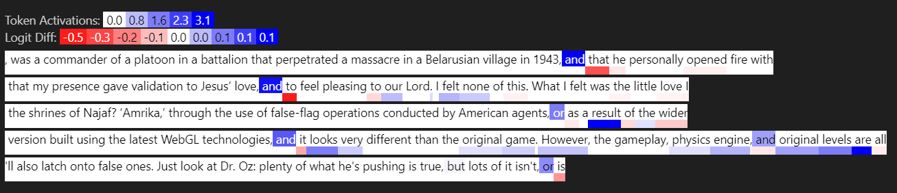
OR Example

In Layer 1, we have:

$O F_{30} = 0.26 I F_{2797} + 0.23 I F_{259} + 0.10 I F_{946}$

where OF is output feature (in MLP_out), and IF is input feature (in Residual Stream before the MLP)

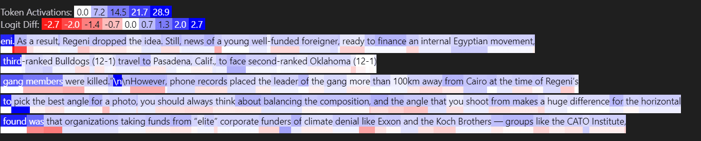
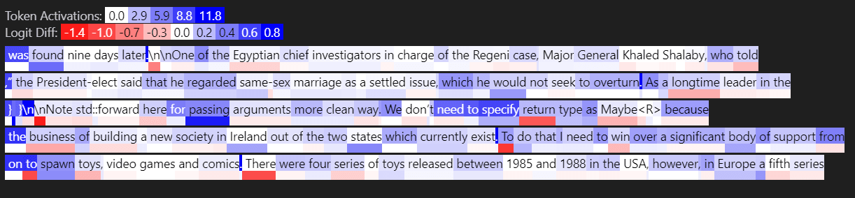
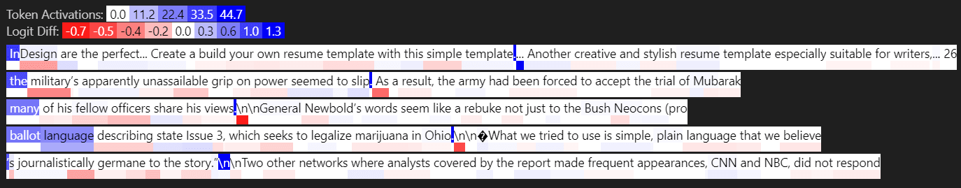
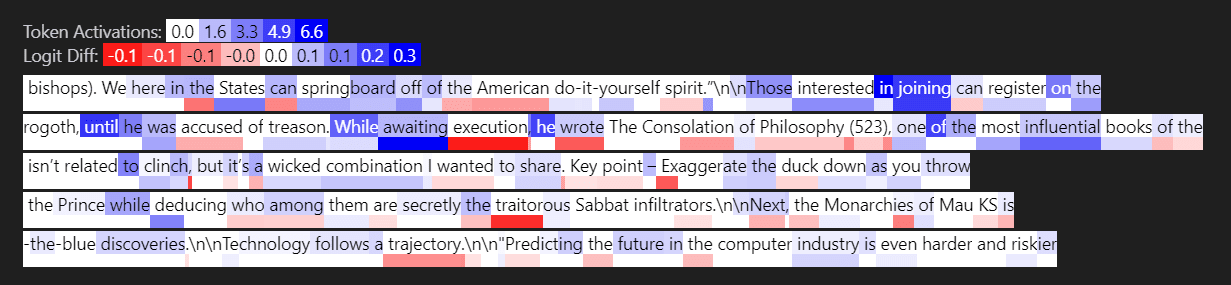
Below is input feature 2797, activating strongly on the token “former”

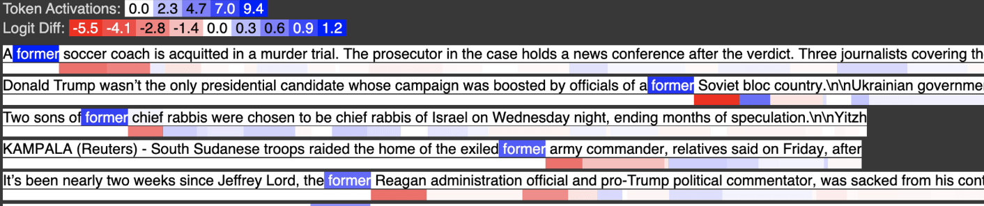
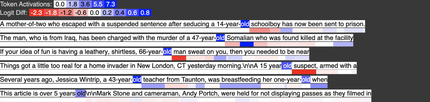
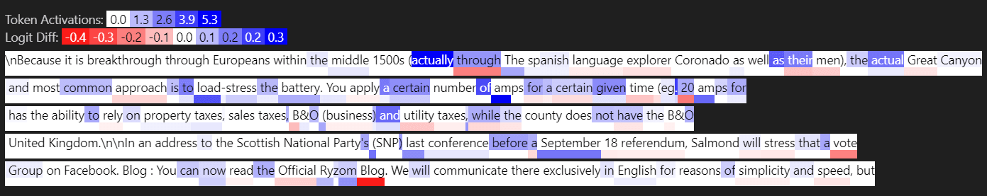
This is 5 examples. For each ex, the top row of words are feature activation e.g. token ” former” activated 9.4. Bottom blank row is: if we removed this feature, how much worse does the model get at predicting these tokens? e.g. Soviet is 5.5 logits worse when the model can’t use this “former” feature.

Below is input feature 259, activating strongly on the token “old”

Below is input feature 946, activating on the token “young”

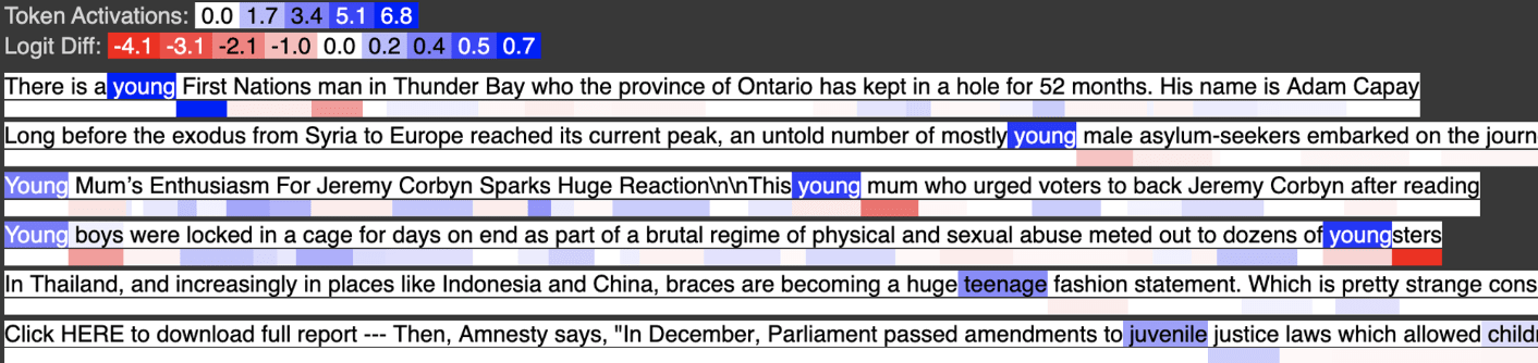
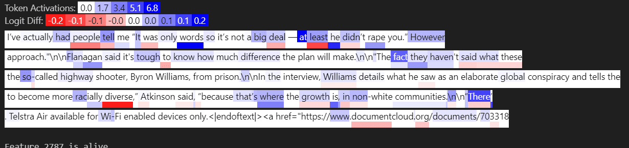
In the output feature, we see the tokens former, old, and young all activate, with young activating about half as strongly as “former” and “old” as we would expect from the weight coefficients.

$O F_{30} = 0.26 F_{f o r m e r} + 0.23 F_{o l d} + 0.10 F_{y o u n g}$

We can view this computation as a weighted logical OR. Output Feature 30 activates on former OR old OR young (again, more examples are here)

Negative Weight Example

In Layer 1, we have:

$O F_{505} = 0.68 I F_{3021} - 0.21 I F_{729}$

where OF is output feature, and IF is input feature.

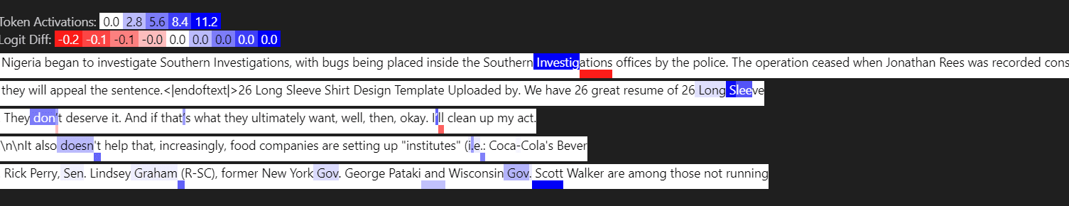
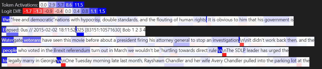
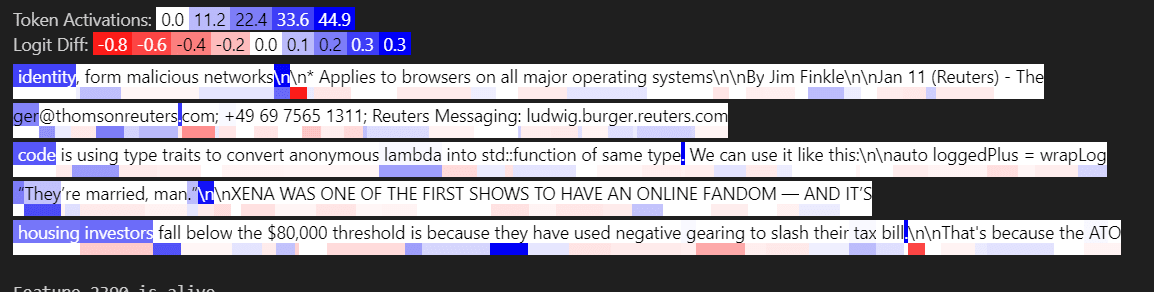
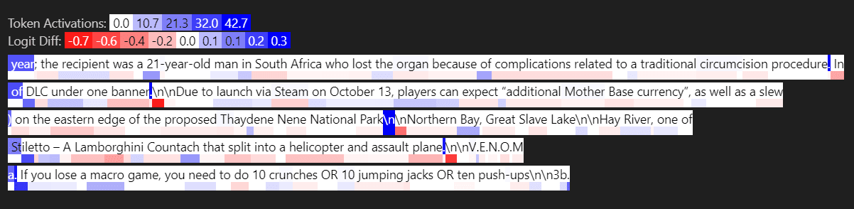
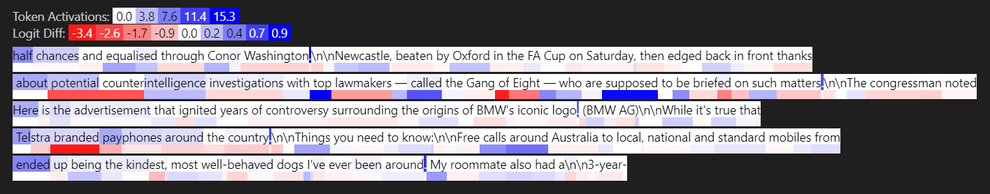
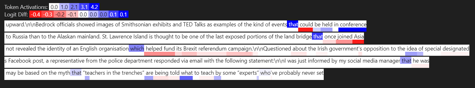
Below is input feature 3021, activating strongly on tokens like “said” which in almost all cases appear not after a quote.

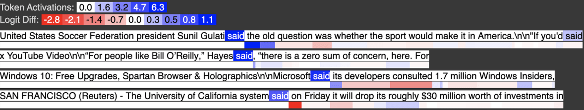
Below is input feature 729, activating strongly on tokens like “said” when they appear shortly after a quote.

Below shows how the activation for input feature 729 changes when we remove a certain context token. Critically, the activation goes does when the quote is removed, demonstrating that this feature activates when there is a quote, followed by “said”.

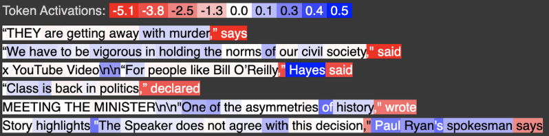
This image typically confuses people. High level take away: anything that is red is important contextual tokens for this feature to activate (the blue isn’t as important because it only adds up to 0.5 when removed, as opposed to −5.1). We’re trying to communicate that removing the quotes makes the feature activation of the word ” says” goes down by −5.1 to 0 feature activation.

Below we see the output feature activates on tokens like “said” that have no prior quote tokens. We’ve “subtracted out” with a large negative weight, so to speak, the examples where “said” appears after a quote, and now the feature only activates when “said” appears without any prior quotes.

$O F_{505} = 0.68 F_{("said" in many contexts)} - 0.21 F_{("said" after quotes)}$

We can view this computation as a weighted logical AND. Output Feature 505 activates on A AND ~B. In the case where A is a superset of B, this is the complement of B e.g. I have the set of all fruits and all yellow fruits, so now I can find all non-yellow fruits.

(again again, more examples are here)

Sparse MLP Feature Connections

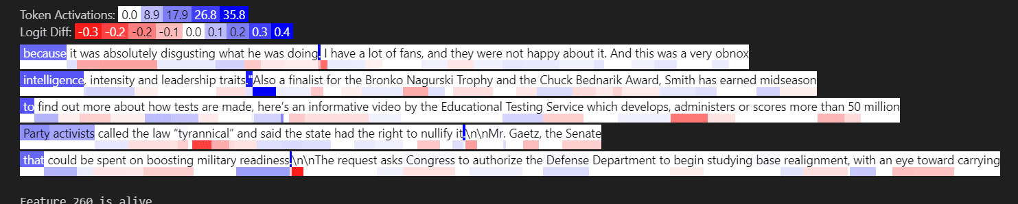
Let’s visualize these MLP features that have the worse losses:

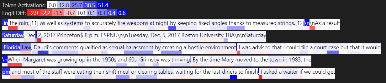
Layer 5: Looking at the features w/ the largest loss-diffs between linear & MLP

(specifically [1.5555, 0.0116, 0.0052, 0.0040, 0.0038])

All 5 features are very high activations. The first one is generally weird (compared to your typical outlier dimension), and the next 4 are mostly weird tokens.

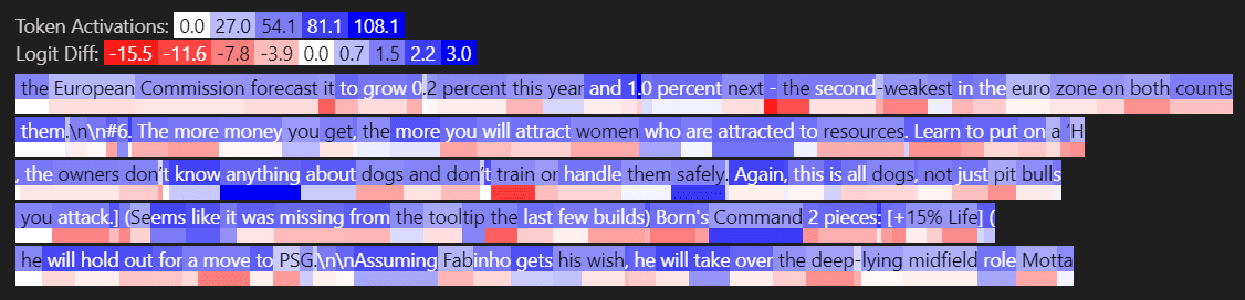
(As a general note: the last layer of LLMs are typically very weird! This also came up for the tuned lens paper, and was hypothesized by nostalgebraist to be an extended unembedding matrix)

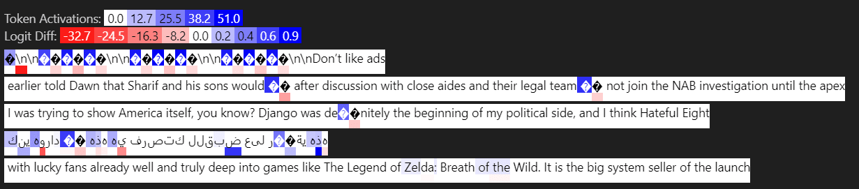
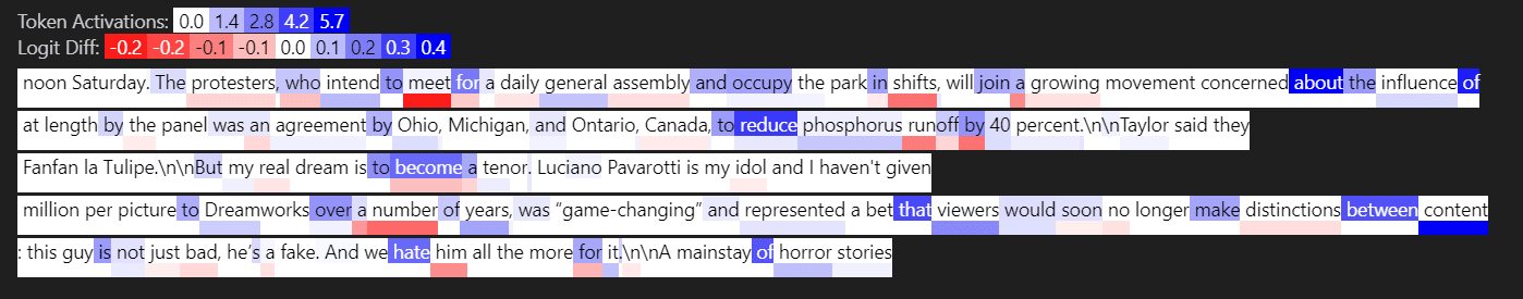
Layer 4: loss-diffs [0.0529, 0.0134, 0.0106, 0.0106, 0.0099]

First & third are outlier features. What is typical for outlier features (from my experience) are:

1) Very high activation (this explains the high L2 loss)

2) Activates on first couple of tokens

3) Activates on first delimiter (e.g. period or newline, which I represent as “\n”)

(Why do these exist? Idk, literature & theories exist, but out of scope for this post)

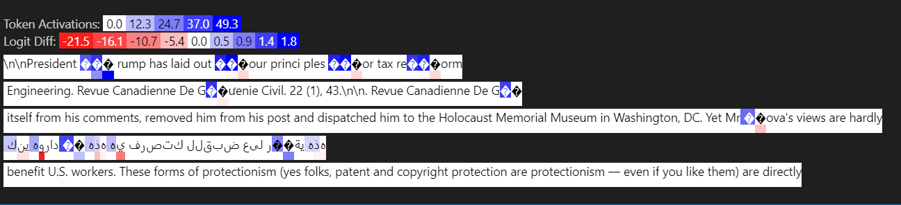
Layer 3: loss-diffs [0.0456, 0.0163, 0.0122, 0.0101, 0.0069]

First & 5th are outlier features

Layer 2: loss-diffs [0.3370, 0.3324, 0.2910, 0.1682, 0.1069]

Four outlier Features

Layer 1: loss-diffs [0.1401, 0.0860, 0.0159, 0.0150, 0.0125]

First Two features are outlier features

What about the specific weights for these features?

So, the MLP has two sets of linear weights: W2(relu(W1(x))). Looking at W2, I noticed the features that had the largest loss had very many large positive & negative weights. Here’s the top 5 loss features (same that are visualized above). For positive weights:

So the highest loss-diff feature in layer 4 had 112 weights connecting it that were > 0.1, where the median feature only had 9.

For negative weights:

Remember these are weights of W2, which connect the LLM’s MLP-out features & the hidden layer of the MLP-connector. We don’t really know what these mean.

But we could definitely just visualize them like we visualize the feature activations, maybe they’re interpretable, so … they were all pretty trash.

Outlier related: ⁸⁄₃₀
Polysemantic: ⁸⁄₃₀
Monosemantic:1/30
(Basically) dead: ¹¹⁄₃₀

(These were for layer 3, but the layer 1 hidden features were surprisingly 80% monosemantic by default, w/ outlier features as well).

Wow, if only we had a method that made hidden layer activations more interpretable! So we could train the sparse MLP connector like a sparse AE: with an l1 penalty on the latent activation (basically an SAE connecting two SAE’s).

SAEs on SAEs

I use the same l1_alpha term for both l1 weights & hidden l1, and see the various losses for Layer 1. Overall:

loss = MSE + L1_alpha*(L1(weights) + L1(hidden_activations))

Losses for various l1_alphas. “Hidden” is L1 loss on hidden activations.

So I picked l1_alpha of 4e-4 as a compromise between MSE & the l1 losses. This corresponded to an L0 of 25 hidden latent activations (ie the other 3k were 0).

Looking at the top 30 max activating features, layer 3, 4, & 5 were all outlier dimensions (first tokens & first delimiter together) for the mlp. The SAE only had 10% outlier features. This makes sense since those outlier dimensions all activate for the same tokens (ie the first tokens & first delimiter), so would have high latent l1 activation. This would incentivize combining those dimensions more.

The features weren’t significantly more monosemantic for the SAE than the MLP. This may be because I need to add a bias for the latent activation. Additionally, I’m confused on how to combine sparse weights w/ sparse latent activations (I specify more in “Help please”). I’ll leave the rest of the empirical work to the future, and proceed w/ speculation.

Interpreting these features could be like the linear AND & OR statements from latent_features → F2. From F1-> latent features is a ReLU, which, w/ a bias would be:

$L a t e n t_F = R e L U (w_{1} f_{1} + w_{2} f_{2} - b i a s)$

specifically

$L a t e n t_F_{3} = R e L U (2.1 * f_{1} + 1.5 * f_{2} - 4)$

This could be either F1 OR F2 if they individually activate more than 4, or F1 AND F2 if they have to both activate together to be greater than 4.

This then makes it important to do feature activation statistics & clustering. It would be good to plot their co-activations (and color according to if it activations the latent feature)

But if I want to do more than 3 features, it’s hard to plot their co-activations. Surely there’s some statistical method here to gather the clusters of co-activations?

Please Help

This was mostly a “go fast & get results” set of experiments, which means many arbitrary choices were made, which I’d appreciate some feedback on. I do intend to research these questions myself (it’s just currently late, and I wanted this post out end of this week).

How should I take in consideration the different norms of the layers when training? For example, Layer 1 has a norm of (7,4) for (residual stream, mlp_out). Layer 5 has one of (16, 54). Atm, I’m dividing MSE by $\frac{(M L P_o u t_{l a y e r}'s norm)^{2}}{min norm}$ , and keeping the weight activation the same.
1. How is this normally handled?
2. How would I handle adding in the latent activation l1 penalty? This isn’t squared, so it would be $\frac{M L P_o u t_{l a y e r}'s norm}{min norm}$ ? I suspect this should consider the MLP_in norm though
3. If I instead normal
Any relevant literature on sparse weightw & sparse latent activation
Stats question: these weight-connections are estimating an estimate (ie the SAE’s are reconstructing the layer’s activations, and the weights are reconstructing the SAE’s reconstruction). Is there some “mean error is the same, but variance is higher” argument here?
What’s the typical tool/algorithm for finding clusters of co-activations? I think correlation is close, but it wouldn’t capture the case of A & B causing the feature, but sometimes A is very large & B is small, and others it’s the reverse.
1. I could also cache all input-feature activations when the latent feature activates, and cluster those. Though I also want input features that cause the latent feature to NOT activate.
2. I also have sparse weights, which should be all the relevant information.

The Grand Plan

If we can define circuits, we can concretely specify important model circuits such as truthfulness, deception, british-english, self-awareness, and personality traits. We will of course argue about if one’s operationalization actually captures what we want, but we would could then actually specify them now to have that argument.

I’m excited about finding features that are causal to each other (this work is correlational). This could be done with gradients or causal interventions. Once we have these causal connections, we still need to find how these features are computed. This work shows many of those connections are linearly computed, and the nonlinearly computed ones are these outlier dimension features (which is useful for an LLM to do text prediction but not useful for model steering).^[2]

For attention features, we can also work on QK/OV circuits between features in the residual stream & those after attention. This also requires taking in consideration feature activation statistics, but seems very doable!

So if we have the connections between features from Residual & MLP_out and Residual & attention_out, then we can also compute the features from the next layer Residual as a sparse linear combination of the previous layer features:
$R_{l a y e r + 1} = R_{l a y e r} + W_{1} * M L P_o u t_{l a y e r} + W_2 * A t t n_o u t_{l a y e r}$

That’s all the connections covered.

There’s plenty of work left to do, but its on the difficulty level of “Normal Academia Can solve it” as opposed to “Prove P !=NP”; this is a much nicer timeline than I thought we were in last year.

If you’d like to work on any Sparse AE projects, feel free to join us on the EleutherAI discord channel (>25k members, so can easily lurk) in the #sparse-coding channel (under interp): https://discord.gg/eleutherai

Feel free to reach out to me (Logan) on discord: loganriggs, dm’s on LW, or the comments below.

Code

For code replication, see my repo at the “static*” files

static-all_sparse_weights—notebook for training & comparing linear vs nonlinear
static-interpret_sparse_weights—notebook for visualizing linear or nonlinear features
static-train_sparse_sae_connector—training the SAE (MLP w/ l1 latent activation penalty)
static-interpre_sparse_weights_mlp—minimal notebook for interpreting the sparse SAE’s latent activations & comparing w/ the MLP’s.

[Note: I haven’t had time to comment or clean up these notebooks. Please message me if you run into any issues]

Appendices

Here are extra experiments that didn’t pan out or were just weird.

Failed MLP sweep

I also tried to reduce the hidden layer size of the MLP, but there was still an increase in MSE. This was without restricting the MLP to only MLP features.

Attention

Also, what if we did the same analysis but on attention?

Layer 4 should be ignored, since it’s mostly dead features, but overall this is pretty weird! I haven’t normalized the loss like I did for MLP, but it seems like many features can be linearly reconstructed by features. This means that attention isn’t really doing attention for a lot of features.

By this I mean attention normally takes in all the features in previous token positions. If we have 200 tokens per example & ~20 features/datapoint, then attention has access to all 20*200 features at the 200th position. Here however, it only has access to the 20 features at the current position. Weird.

^
Additionally, the full computation between features F1 & F2 must include the decoder from SAE_1, the MLP, & encoder + ReLU from SAE_2.
F2 = relu(linear(linear(gelu(linear(linear(F1))))))
= relu(linear(gelu(linear(F1))) [Since two linear functions can be equivalent to 1 linear function)
^
I do think it’d be valuable to figure out what causal role these outlier dimensions play.

Finding Sparse Linear Connections between Features in LLMs