Computing Natural Abstractions: Linear Approximation
Background: Testing The Natural Abstraction Hypothesis
Given a world-model, direct computation of natural abstractions basically amounts to figuring out which -values give the same -distributions , for various choices of the variables and in some large Bayes net. In general, this computation is #P-Hard. (That’s like NP-Hard, but Harder.) That doesn’t necessarily mean that it’s usually intractable in practice, but it means that we need to use heuristics and approximations right off the bat.
A linear-Guassian approximation is a natural starting point. It’s relatively simple—all of the relevant computations are standard matrix operations. But it’s also relatively general: it should be a good approximation for any system with smooth dynamics and small noise/uncertainty. For instance, if our system is a solid object made of molecules and sitting in a heat bath, then linear-Gaussian noise should be a good model. (And that’s a good physical picture to keep in mind for the rest of this post—solid object made of molecules, all the little chunks interacting elastically, but also buffeted about by thermal noise.)
So, we have some Bayes net in which each variable is Gaussian—a linear combination of its parents plus some IID Gaussian noise. For the underlying graph, I’m using a 2D Delaunay triangulation, mainly because it does a good job reflecting physically-realistic space/time structure. (In particular, as in physical space, most pairs of nodes are far apart—as opposed to the usual Erdos-Renyi random graph, where the distance between most points is logarithmic. We’ll revisit the choice of graph structure later.) Embedded in 2D, an example graph looks like this:
… although the actual experiments below will use a graph with about 500X more nodes (50k, whereas the visual above uses 100). Each of those nodes is a Gaussian random variable, with the arrows showing its parents in the Bayes net. Weights on the edges (i.e. coefficients of each parent) are all random normal, with variance ⅔ (another choice we’ll revisit later).
Let’s start with the basic experiment: if we pick two far-apart neighborhoods of nodes, and , can the information from which is relevant to fit into a much-lower-dimensional summary? In a Gaussian system, we can answer this by computing the covariance matrix , taking an SVD, and looking at the number of nonzero singular values. Each left singular vector with a nonzero singular value gives the weights of one variable in the “summary data” of which is relevant to . (Or, for information in relevant to , we can take the right singular vectors; the dimension of the summary is the same either way.)
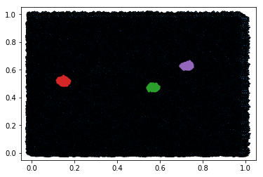
We’ll use these three randomly-chosen neighborhoods of nodes (green is neighborhood 1, red is 2, purple is 3):
Here are the 10 largest singular values of the neighborhood 1 - neighborhood 2 covariance matrix:
array([5.98753213e+05, 1.21862101e+02, 1.91973783e-01, 1.03200621e-03,
       2.01888771e-04, 1.05877548e-05, 5.34855466e-06, 4.94833571e-10,
       2.55557198e-10, 2.17092875e-10])
The values of order 1e-10 or lower are definitely within numerical error of zero, and I expect the values of order 1e-3 or lower are as well, so we see at most 7 nonzero singular values and probably more like 3. (I know 1e-3 seems high for numerical error, but the relevant number here is the ratio between a given singular value and the largest singular value, so it’s really more like 1e-8. In principle a double provides 1e-16 precision, but in practice it’s common to lose half the bits in something like SVD, and 1e-8 is about how much I usually trust these things.) Meanwhile, the two neighborhoods contain 109 and 129 nodes, respectively.
To summarize all that: we picked out two neighborhoods of ~110 variables each in a 50k-node linear Gaussian network. To summarize all the information from one neighborhood relevant to the other, we need at most a 7-variable summary (which is also linear and Gaussian). That’s already a pretty interesting result—the folks at SFI would probably love it.
But it gets even better.
We can do the same thing with the neighborhood 1 - neighborhood 3 covariance matrix. The first 10 singular values are:
array([7.50028046e+11, 5.87974398e+10, 2.50629095e+08, 2.23881004e+03,
       1.46035030e+01, 2.52752074e+00, 1.01656991e-01, 1.79916658e-02,
       5.89831843e-04, 3.52074803e-04])
… and by the same criteria as before, we see at most 8 nonzero singular values, and probably more like 3. Now, we can compare the neighborhood-1-singular-vectors from our two SVDs. Simply computing the correlations between each pair of nonzero singular vectors from the two decompositions yields:
Key thing to notice here: the first two singular vectors are near-perfectly correlated! (Both correlations are around .996.) The correlations among the next few are also large, after which it drops off into noise. (I did say that everything after the first three singular components was probably mostly numerical noise.)
In English: not only can a three-variable summary of neighborhood 1 probably contain all the info relevant to either of the other two neighborhoods, but two of the three summary variables are the same.
This is exactly the sort of thing the natural abstraction hypothesis predicts: information relevant far away fits into a compact summary—the “abstract summary”—and roughly-the-same abstract summary is relevant even from different “vantage points”. Or, to put it differently, the abstraction is reasonably robust to changes in which “far away” neighborhood we pick.
Our 2D-embedded linear-Gaussian world abstracts well.
Of course, this was just an example from one run of the script, but the results are usually pretty similar—sometimes the summary has 2 or 4 or 5 dimensions rather than 3, sometimes more or fewer summary-dimensions align, but these results are qualitatively representative. The main case where it fails is when the RNG happens to pick two neighborhoods which are very close or overlap.
Is This Just The Markov Blanket?
Notice that our “neighborhoods” of variables include some nodes strictly in the interior of the neighborhood. The variables on the boundary of the neighborhood should form a Markov blanket—i.e. they are themselves an abstract summary for the whole neighborhood, and of course they’re the same regardless of which second neighborhood we pick. So perhaps our results are really just finding the variables on the neighborhood boundary?
The results above already suggest that this is not the case: we can see at a glance that the dimension of the summary is quite a bit smaller than the number of variables on the boundary. But let’s run another test: we’ll fix the point at the “center” of the neighborhood, then expand the neighborhood’s “radius” (in terms of undirected steps in the graph), and see how both the boundary size and the summary size grow.
Here are results from one typical run (number of boundary variables in blue, number of summary variables in red):
As we expand the neighborhood, the number of boundary-variables grows, but the number of summary variables stays flat. So there’s definitely more going on here than just the neighborhood’s Markov blanket (aka boundary variables) acting as an abstract summary.
What About…
The above toy model made two choices which one could imagine not generalizing, even in other sparse linear-Gaussian systems.
First, the graph structure. The random graphs most often used in mathematics are Erdos-Renyi (ER) random graphs. “Information relevant far away” doesn’t work very well on these, because nodes are almost never far apart. The number of steps between the two most-distant nodes in such graphs is logarithmic. So I wouldn’t expect environments with such structure to abstract well. On the other hand, I would usually expect such environments to be a poor model for systems in our physical world—the constraints of physical space-time make it rather difficult to have large numbers of variables all interacting with only logarithmic causal-distances between them. In practice, there are usually mediating variables with local interactions. Even the real-world systems which most closely resemble ER random graphs, like social networks or biochemical regulatory networks, tend to have much more “localized” connections than a true ER random graph—e.g. clusters in social networks or modules in biochemical networks.
(That said, I did try running the above experiments with ER graphs, and they work surprisingly well, considering that the neighborhoods are only a few steps apart on the graph. Summary sizes are more like 10 or 12 variables rather than 2 or 4, and alignment of the summary-variables is hit-and-miss.)
Second, the weights. There’s a phase shift phenomenon here: if the weights are sufficiently low, then noise wipes out all information over a distance. If the weights are sufficiently high, then the whole system ends up with one giant principal component. Both of these abstract very well, but in a boring-and-obvious way. The weights used in these experiments were chosen to be right at the boundary between these two behaviors, where more interesting phenomena could potentially take place. If the system abstracts well right at the critical point, then it should abstract well everywhere.
So What Could We Do With This?
I mainly intend to use this sort of model to look for theoretical insights into abstraction which will generalize beyond the linear-Gaussian case. Major goals include data structures for representing whole sets of abstractions on one environment, as well as general conditions under which the abstractions are learned by a model trained on the environment.
But there are potential direct use-cases for this kind of technique, other than looking for hints at more-general theory.
One example would be automatic discovery of abstractions in physical systems. As long as noise is small and the system is non-chaotic (so noise stays small), a sparse linear-Gaussian model should work well. (In practice, this mainly means the system needs to have some kind of friction in most degrees of freedom.) In this case, I’d expect the method used here to work directly: just compute covariances between far-apart neighborhoods of variables, and those covariances will likely be low-rank.
In principle, this method could also be directly applied to machine learning systems, although the range of applicability would be fairly narrow. It would only apply to systems where linear approximations work very well (or maybe quadratic approximations, which give a linear approximation of the gradient). And ideally the random variables would be Gaussian. And it should have a fairly large and deep computational graph, so most neighborhoods of variables are not too close together. If one just happened to have an ML model which met those criteria, we’d expect these results to carry over directly: compute the covariance matrix between far-apart neighborhoods of the random variables in the model, and those matrices should be low-rank. That sounds like a potentially-very-powerful transparency tool… if one had a model which fit the criteria. Hypothetically.
Summary
Build a random linear-Gaussian Bayes net with a random planar graph structure (in this case generated from a Delaunay mesh). Pick two far-apart neighborhoods of variables in this net, and use an SVD to compute the rank of their covariance matrix. Empirically, we find rank <10 even with 110-variable neighborhoods in a 50k-node network. In other words: a very small number of variables typically suffices to summarize all the information from a neighborhood of variables which is relevant far away. The system abstracts well.
Furthermore: the largest singular vectors are the same even for different choices of the second (far-away) neighborhood. Not only does a small summary suffice, but approximately the same small summary suffices. The abstractions are robust to changes in our “far away” reference neighborhood.
- Natural Abstractions: Key Claims, Theorems, and Critiques by (16 Mar 2023 16:37 UTC; 250 points)
- Testing The Natural Abstraction Hypothesis: Project Update by (20 Sep 2021 3:44 UTC; 88 points)
- [AN #148]: Analyzing generalization across more axes than just accuracy or loss by (28 Apr 2021 18:30 UTC; 24 points)
- 's comment on Testing The Natural Abstraction Hypothesis: Project Intro by (23 Apr 2021 21:39 UTC; 4 points)
- 's comment on Testing The Natural Abstraction Hypothesis: Project Update by (14 Aug 2022 15:28 UTC; 3 points)
- 's comment on Prize for Alignment Research Tasks by (16 May 2022 5:21 UTC; 1 point)
What a small world—I was thinking up a very similar transparency tool since two weeks ago. The function f from inputs to activations-of-every-neuron isn’t linear but it is differentiable, aka linear near (input space, not pixel coordinates!) an input. The jacobian J at an input x is exactly the cross-covariance matrix between a normal distribution 𝓝(x,Σ) and its image 𝓝(f(x),JΣJᵀ), right? Then if you can permute a submatrix of JΣJᵀ into a block-diagonal matrix, you’ve found two modules that work with different properties of x. If the user gives you two modules, you could find an input where they work with different properties, and then vary that input in ways that change activations in one module but not the other to show the user what each module does. And by something like counting the near-zero entries in the matrix, you could differentiably measure the network’s modularity, then train it to be more modular.
Train a (GAN-)generator on the training inputs and attach it to the front of the network—now you know the input distribution is uniform, the (reciprocals of) singular values say the density of the output distribution in the direction of their singular vector, and the inputs you show the user are all in-distribution.
And I’ve thought this up shortly before learning terms like cross-covariance matrix, so please point out terms that describe parts of this. Or expand on it. Or run away with it, would be good to get scooped.
With differential geometry, there’s probably a way to translate properties between points. And a way to analyze the geometry of the training distribution: Train the generator to be locally injective and give it an input space uniformly distributed on the unit circle, and whether it successfully trains tells you whether the training distribution has a cycle. Try different input topologies to nail down the distribution’s topology. But just like J’s rank tells you the dimension of the input distribution if you just give the generator enough numbers to work with, a powerful generator ought to tell you the entire topology in one training run...
If the generator’s input distribution is uniform, Σ is diagonal, and the left SVD component of J is also the left (and transposed right) SVD component of JΣJᵀ. Is that useful?
I’d be curious to know whether something like this actually works in practice. It certainly shouldn’t work all the time, since it’s tackling the #P-Hard part of the problem pretty directly, but if it works well in practice that would solve a lot of problems.
Also, question, one way that you can get an abstraction of the neighbourhood is via SVD between the neighbourhood’s variables and other variables far away, but another way that you can do it is just by applying PCA on the variables in the neighbourhood itself. Does this yield the same result, or is there some difference? My guess would be that it would yield highly correlated variables to what you get from SVD.
Finally, intuitively from intuition on PCA, I would assume that the most important variable would tend to correspond to some sort of “average activation” in the neighbourhood, and the second most important variable would tend to correspond to the difference between the activation in the top of the neighbourhood and the activation in the bottom of the neighbourhood. Defining this precisely might be a bit hard, as the signs of nodes are presumably somewhat arbitrary, so one would have to come up with some way to adjust for that; but I would be curious if this looks anything like what you’ve found?
I guess in a way both of these hypotheses contradict your reasoning for why the natural abstraction hypothesis holds (though is quite compatible with it still holding), in the sense that your natural abstraction hypothesis is built on the idea that noisy interactions just outside of the neighbourhood wipe away lower-level details, while my intuitions are that a lot of the information needed for abstraction could be recovered from what is going on within the neighbourhood.
I’ve been thinking a fair bit about this question, though with a slightly different framing.
Let’s start with a neighborhood X. Then we can pick a bunch of different far-away neighborhoods Y1,...,Yn, and each of them will contain some info about summary(X). But then we can flip it around: if we do a PCA on (X,Y1,...,Yn), then we should expect to see components corresponding to summary(X), since all the variables which contain that information will covary.
Switching back to your framing: if X itself is large enough to contain multiple far-apart chunks of variables, then a PCA on X should yield natural abstractions (roughly speaking). This is quite compatible with the idea of abstractions coming from noise wiping out info: even within X, noise prevents most info from propagating very far. The info which propagates far within X is also the info which is likely to propagate far beyond X itself; most other info is wiped out before it reaches the boundaries of X, and has low redundancy within X.
Agree, I was mainly thinking of whether it could still hold if X is small. Though it might be hard to define a cutoff threshold.
Perhaps another way to frame it is, if you perform PCA, then you would likely get variables with info about both the external summary data of X, and the internal dynamics of X (which would not be visible externally). It might be relevant to examine things like the relative dimensionality for PCA vs SVD, to investigate how well natural abstractions allow throwing away info about internal dynamics.
(This might be especially interesting a setting where it is tiled over time? As then the internal dynamics of X play a bigger role in things.)
🤔
That makes me think of another tangential thing. In a designed system, noise can often be kept low, and redundancy is often eliminated. So the PCA method might work better on “natural” (random or searched) systems than on designed systems, while the SVD method might work equally well on both.
Did you set up your previous posts with this experiment in mind? I had been toying with some similar things myself, so it’s fun to see your analysis too.
Regarding choices that might not generalize, another one that I have been thinking about is agency/optimization. That is, while your model is super relevant for inanimate systems, optimized systems often try to keep some parameters under control, which involves many parameters being carefully adjusted to achieve that.
This might seem difficult to model, but I have an idea: Suppose you pick a pair of causal nodes X and Y, such that X is indirectly upstream from Y. In that case, since you have the ground truth for the causal network, you can compute how to adjust the weights of X’s inputs and outputs to (say) keep Y as close to 0 as possible. This probably won’t make much of a difference when picking only a single X, but for animate systems a very large number of nodes might be set for the purpose of optimization. There is a very important way that this changes the general abstract behavior of a system, which unfortunately nobody seems to have written about, though I’m not sure if this has any implications for abstraction.
Also, another property of the real world (that is relatively orthogonal to animacy, but which might interact with animacy in interesting ways) that you might want to think about is recurrence. You’ve probably already considered this, but I think it would be interesting to study what happens if the causal structure tiles over time and/or space.
If matrix A maps each input vector of X to a vector of which the first entry corresponds to Y, subtracting multiples of the first row from every other row to make them orthogonal to the first row, then deleting the first row, would leave a matrix whose row space is the input vectors that keep Y at 0, and whose column space is the outputs thus still reachable. If you fix some distribution on the inputs of X (such as the normal distribution with a given covariance matrix), whether this is losslessly possible should be more interesting.
Presumably you wouldn’t be able to figure out the precise value of Y since Y isn’t connected to X. You could only find an approximate estimate. Though on reflection the outputs are more interesting in a nonlinear graph (which was the context where I originally came up with the idea), since in a linear one all ways of modifying Y are equivalent.
All ways of modifying Y are only equivalent in a dense linear system. Sparsity (in a high-dimensional system) changes that. (That’s a fairly central concept behind this whole project: sparsity is one of the main ingredients necessary for the natural abstraction hypothesis.)
I think I phrased it wrong/in a confusing way.
Suppose Y is unidimensional, and you have Y=f(g(X), h(X)). Suppose there are two perturbations i and j that X can emit, where g is only sensitive to i and h is only sensitive to j, i.e. g(j)=0, h(i)=0. Then because the system is linear, you can extract them from the rest:
Y=f(g(X+ai+bj), h(X+ai+bj))=f(g(X), h(X))+af(g(i))+bf(h(j))
This means that if X only cares about Y, it is free to choose whether to adjust a or to adjust b. In a nonlinear system, there might be all sorts of things like moderators, diminishing returns, etc., which would make it matter whether it tried to control Y using a or using b; but in a linear system, it can just do whatever.
Oh I see. Yeah, if either X or Y is unidimensional, then any linear model is really boring. They need to be high-dimensional to do anything interesting.
They need to be high-dimensional for the linear models themselves to do anything interesting, but I think adding a large number of low-dimensional linear models might, despite being boring, still change the dynamics of the graphs to be marginally more realistic for settings involving optimization. X turns into an estimate of Y, and tries to control this estimate towards zero; that’s a pattern that I assume would be rare in your graph, but common in reality, and it could lead to real graphs exhibiting certain “conspiracies” that the model graphs might lack (especially if there are many (X, Y) pairs, or many (individually unidimensional) Xs that all try to control a single common Y).
But there’s probably a lot of things that can be investigated about this. I should probably be working on getting my system for this working, or something. Gonna be exciting to see what else you figure out re natural abstractions.
Y can consist of multiple variables, and then there would always be multiple ways, right? I thought by indirect you meant that the path between X and Y was longer than 1. If some third cause is directly upstream from both, then I suppose it wouldn’t be uniquely defined whether changing X changes Y, since there could be directions in which to change the cause that change some subset of X and Y.
Not necessarily. For instance if X has only one output, then there’s only one way for X to change things, even if the one output connects to multiple Ys.
Yes.
I’m not sure I get it, or at least if I get it I don’t agree.
Are you saying that if we’ve got X ← Z → Y and X → Y, then the effect of X on Y may not be well-defined, because it depends on whether the effect is through Z or not, as the Z → Y path becomes relevant when it is through Z?
Because if so I think I disagree. The effect of X on Y should only count the X → Y path, not the X ← Z → Y path, as the latter is a confounder rather than a true causal path.
The main thing I expect from optimization is that the system will be adjusted so that certain specific abstractions work—i.e. if the optimizer cares about f(X), then the system will be adjusted so that information about f(X) is available far away (i.e. wherever it needs to be used).
That’s the view in which we think about abstractions in the optimized system. If we instead take our system to be the whole optimization process, then we expect many variables in many places to be adjusted to optimize the objective, which means the objective itself is likely a natural abstraction, since information about it is available all over the place. I don’t have all the math worked out for that yet, though.
Another question:
It seems to me like with 1 space dimension and 1 time dimension, different streams of information would not be able to cross each other. Intuitively the natural abstraction model makes sense and I would expect this stuff to work with more space dimensions too—but just to be on the safe side, have you verified it in 2 or 3 spatial dimensions?
(… 🤔 isn’t there supposedly something about certain properties undergoing a phase shift beyond 4 dimensions? I have no idea whether that would come up here because I don’t know the geometry to know the answer. I assume it wouldn’t make a difference, as long as the size of the graph is big enough compare to the number of dimensions. But it might be fun to see if there’s some number of dimensions where it just completely stops working.)
Well, it worked reasonably well with ER graphs (which naturally embed into quite high dimensions), so it should definitely work at least that well. (I expect it would work better.)
I second Tailcalled’s question, and would precisify it: When did you first code up this simulation/experiment and run it (or a preliminary version of it)? A week ago? A month ago? Three months ago? A year ago?
I ran this experiment about 2-3 weeks ago (after the chaos post but before the project intro). I pretty strongly expected this to work much earlier—e.g. back in December I gave a talk which had all the ideas in it.
Note to self: the summary dimension seems basically constant as the neighborhood size increases. There’s probably a generalization of Koopman-Pitman-Darmois which applies.
This seems like it would be unlikely to hold in 2 or 3 dimensions?