Translating between Latent Spaces
Produced as part of the SERIMATS Program 2022 Research Sprint under John Wentworth
Introduction
The gold-standard of interpretability in ML systems looks like finding embeddings of human-identifiable concepts in neural net architectures, and being able to modify, change, and activate them as we wish. The first hurdle is identification of these concepts. We propose that it may be easier to identify simpler concepts in simpler models, and use these to bootstrap to more complex concepts in more intricate models.
To this end, we first propose a definition of what it means for a concept to be present in a model. Then we investigate how we can identify similar concepts across different models. We begin by demonstrating these definitions and techniques in a simple example involving Bayes nets.
We then train two autoencoders (small and large) on the FashionMNIST dataset. We choose some latent concepts that humans would use to represent shoes (shoe height and shoe brightness) and see whether these human concepts can be transferred to the models, and how the models’ representations relate.
A simple example
Simple Environment
First we construct a simple environment:
There are 10 cells.
Each cell can contain nothing, a blue circle, a red circle, or both.
There is one red circle.
The red circle moves 1 right each timestep.
If the red circle cannot move right, it moves to the leftmost cell.
There are two adjacent blue circles.
The blue circles move 1 left or 1 right each timestep.
If a blue circle reaches the environment’s edge, both their directions change.
If a cell contains a red circle and a blue circle, it shows only a blue circle.
A sample is given below:
Two Models of this Environment
We model the evolution of this environment using two different Bayes nets. Each Bayes net reflects a different way of viewing this environment corresponding to:
An object centric model
A local-state centric model
Object Centric Model (Model 1)
The object centric model tracks 3 latent variables corresponding to the object-level description of where the blue and red circles are and in which direction the blue circles are moving at a given timestep:
blue location (taking values in )
red location (taking values in )
blue velocity (taking values in )
It also has 10 observational variables given by the 10 cells, which take values in .
This is represented by the following Bayes net (each column being a new timestep):
So this Bayes net has a latent space given by the set , and the state displayed at timestep 2 in the above diagram would have (assuming blue is moving right) latent representation .
Local-State Centric Model (Model 2)
The local-state centric model treats each cell as having a local state corresponding to
Whether the cell contains a red circle
Whether the cell contains a blue circle
If the cell contains a blue circle, which direction the blue circle is moving in
So each cell can be in one of six possible states:
No Red, No Blue -
Red, No Blue -
No Red, Blue moving left -
Red, Blue moving left -
No Red, Blue moving right -
Red, Blue moving right -
And this is represented by the Bayes net:
So the latent space of this Bayes net consists of tuples from the set , and the state displayed at timestep 1 would have (assuming blue is moving right) latent representation .
Definitions
Now that we have an environment and two simple models to refer to, let’s define some notions that will be useful:
A latent concept is an abstract concept which changes across the training data. Some examples in the above environment: ‘blue direction,’ ‘location of the blue circle,’ ‘location of all three circles,’ and ‘state of the 3rd cell.’ (Due to the simple nature of the above environment, all of these latent concepts take values in discrete sets, but latent concepts can be continuous as well.)
Relationship components take latent concepts as input, and output how these change other latent concepts in the model. They do this by representing operations or functions that are constant across the training data. In the above example, this might be ‘the red circle always moves right’ or ‘the blue circles bounce off the edge.’
A latent concept identifier takes as input a vector in the latent space of a model, and outputs the value of the latent concept being measured.
These concepts at work in Bayes nets
We will choose ‘blue velocity’ as our latent concept and establish a latent concept identifier for blue velocity in the object centric Bayes net. Then we want to use this latent concept identifier to communicate this latent concept from the object centric latent space to the local-state centric latent space and hence derive the latent concept identifier in this new latent space.
The latent concept identifier function for blue velocity in the object centric Bayes net is obvious by inspection, it is simply:
such that
,
since this concept is represented directly in the third coordinate of the latent space.
The second latent space stores this same concept in a noticeably more indirect and distributed way, and the latent concept identification function is correspondingly more complex.
such that
This function would be easy to learn from example data using a decision tree or neural net. This would be done by generating observation sequences using the object centric Bayes net, then obtaining the corresponding latent state using the local-state Bayes net, and labelling it using the object-centric concept identifier and latent state. The process of learning this function constitutes the transferring of the latent concept from the first latent space to the second latent space which was what we hoped to achieve.
The complete-data limit
We now take the general method sketched out in the example above, and formalize it. We aim to show that for 2 models, when we can compare the latent concepts across all possible inputs to the models, we can perfectly communicate latent concepts from one model to another.
Let’s define:
A set of observations , in humans this is the set of all possible sequences of sense-data over a lifetime, in the Bayes net example above it’s .
Two spaces and which represent the latent spaces of two world models.
Two functions, and , to represent each world model. Each function maps observations to latent states, . Assume that these world models were trained as generative models to predict any part of the observation given any other part of the observation, so it uses the latent space to store any information relevant to predicting any potential observation.
Now we have a concept, say “blue velocity”, which we define using a function .
Our goal is to successfully communicate a concept from one model to the other. In other words, to discover the function , such that:
If we assume is invertible.[1]
Then we can define as:
for any .
A similar approach to the above can be used to learn a latent concept identifier that is invertible, i.e. we can use it to manipulate the belief state of the world model. In that case we need to also iterate over possible changes to latent state 1 which match the predictions made by world model 2 when the relevant latent variable is changed.
Variational Autoencoders (VAEs) trained on FashionMNIST
Now we consider a more complex example involving neural nets. We train two variational autoencoders on the FashionMNIST dataset. A variational autoencoder is made up of two components: an encoder and a decoder. The encoder is trained to take in an image and map it to a point in an -dimensional latent space. The decoder is simultaneously trained to take these points in the latent space, and reconstruct an image that minimises binary cross-entropy loss between the actual image and what the decoder predicts the image to look like from knowing where the encoder sends it.
VAE FashionMNIST representations
Below are two plots of the latent spaces of variational autoencoders trained with a 2D latent space:
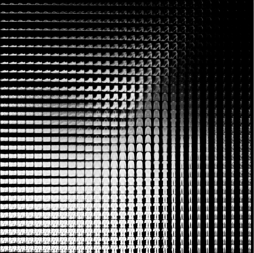
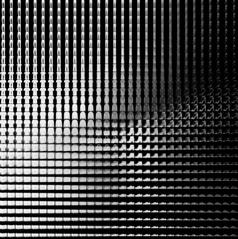
We can see that there are regions of the space that correspond to concepts we might use ourselves to represent fashion items. For example, the top left region in the first latent space, and bottom right region in the second latent space are both ‘shoe-regions’ in their respective latent spaces. And they seem to be clustered in a fairly sensible way!
There are also regions of these latent spaces that clearly do not correspond to ways we would think about fashion items: an example that occurs in almost every latent space we generated is t-shirts turning into pants, and we can see that both latent spaces store weird half t-shirt, half pants images.
Therefore, we’re not looking for every concept that the autoencoder uses to represent fashion items to be analogous to human representations of fashion items. But we are looking for the reverse implication to hold: that human representations of fashion items will have an analogous representation in these latent spaces. Moreover, this holds only for local concepts since global concepts like “formality of fashion items” will not be learnt by the autoencoder, but we would expect local concepts like ‘height of shoe’ or ‘brightness of shirt’ to be learnt.
VAEs with Higher Dimensional Latent Spaces
We train two slightly different VAE models of different sizes, a smaller and a larger one. Each model has 20 latent space dimensions, but after training we found that a smaller number of dimensions are used in practice. The number of dimensions used was fairly consistent between different runs. For the smaller model, usually only 5 were used (though sometimes 6). For the larger model, usually 10 were used (sometimes 9). Increasing the number of dimensions in the latent space also had little effect on the number of dimensions the model learns to use.
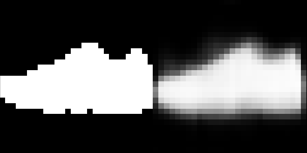
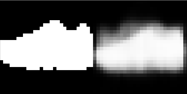
We use these VAEs to encode two artificially whitened out shoes, and then decode them to see where they get sent. The first whitened out shoe was obtained by selecting a shoe from the dataset, and rounding all the pixel values. The second shoe was obtained by manually adding two white pixels on top of this shoe. Our hope was that this would eliminate other variables (e.g. texture) that might interfere with how the VAEs encode shoes, and that thereby we could determine a vector along which ‘shoe height’ is varying.
Shoe encodings (and decodings)
Regular size shoe, and what the model generates from its encoding:
Shoe +2 pixels to height, and what the model generates from its encoding:
Does this give us a vector corresponding to shoe height?
We took this vector along which (we hope) shoe height was varying, normalized it, and plotted images at different points along this vector (taking the origin to be the first encoded shoe) and obtained:
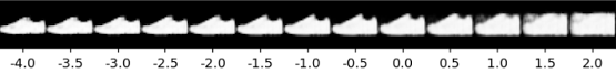
This movement in latent space locally corresponds to shoe height. When we extrapolate far enough in any direction, it will ultimately reach a region of latent space which does not correspond to any human-interpretable concept (c.f. the bottom left region of the two dimensional example latent spaces), so this local behaviour is the best we could hope for.
Now let’s vary the same vector about an example of a real encoded shoe. This should show to what extent this direction corresponds to shoe height (although VAEs map concepts non-linearly, so it will be at best a good local approximation of increasing shoe height):
And again it does seem to correspond (roughly) to shoe height.
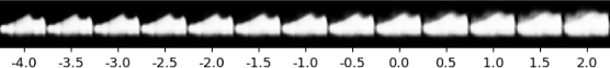
Larger VAE
We then apply this procedure to the larger VAE, and generate corresponding images that (we hope) vary just in shoe height. In this VAE, however, moving along the height vector also increases brightness. (especially noticeable in the second image below, but present in both):
Orthogonal vectors in latent space
We then investigate whether we can separate the model’s learnt concept for brightness from its learnt concept for shoe height:

Some brief attempts were tried by first getting a vector for brightness and then a vector orthogonal to this (using Gram-Schmidt), but this didn’t quite work. Depending on how one increased brightness, one could get a vector that is not orthogonal to shoe height. For the larger VAE, moving along the brightness vector, the shoe gets both brighter and taller than in the shoe height direction—our orthogonalization attempts unfortunately did not end up working.
Directions worth further research
The sample efficiency of learning a latent concept identifier should depend on the similarity of the abstractions used by each model. Can we demonstrate this? Can we make progress on this by assuming some version of the natural abstraction hypothesis?
How do we formalize learning latent concept identifiers to cases where we are transferring from a better model to a worse model of the world (i.e. when is not invertible)?
How do we extend learning latent concept identifiers to cases where both models are imperfect in different ways: where one model is better at predicting some types of observations but is beaten on others?
Can we isolate independent directions in the latent space of variational autoencoders that actually represent identifiable concepts orthogonally?
Can we find similar behaviour in larger autoencoders of more complex datasets? Will increasing the number of parameters and complexity of data serve to make represented concepts more human-identifiable, or less?
- ^
Note that this is a strong assumption, it implies that any observation sequence leads to a unique “belief state” about the world. I.e. it’s a lossless representation of the world. The assumption makes sense for perfectly modelled deterministic environments.
I’d be interested to hear you elaborate on exactly how these attempts failed. What goes wrong if you look at vectors of the form vb+αvh for α∈R and vb,vh the vectors in latent space that you identify for brightness and height respectively, and then do some kind of manual binary search on α to eyeball the value that cancels out the brightness factor? Do you run into a collinearity problem when you try this, for instance?
Some literature which might be useful: Cross-GAN Auditing: Unsupervised Identification of Attribute Level Similarities and Differences between Pretrained Generative Models; LatentCLR: A Contrastive Learning Approach for Unsupervised Discovery of Interpretable Directions.