(Work done as part of SERI MATS Summer 2023 cohort under the supervision of @Lee Sharkey . A blog post containing audio features that you can listen to can be found here.)

TL;DR—Mechanistic Interpretability has mainly focused on language and image models, but there’s a growing need for interpretability in multimodal models that can handle text, images, audio, and video. Thus far, there have been minimal efforts directed toward interpreting audio models, let alone multimodal ones. To the best of my knowledge, this work presents the first attempt to do interpretability on a multimodal audio-text model. I show that acoustic features inside OpenAI’s Whisper model are human interpretable and formulate a way of listening to them. I then go on to present some macroscopic properties of the model, specifically showing that encoder attention is highly localized and the decoder alone acts as a weak LM.

Why we should care about interpreting multimodal models

Up to this point, the main focus in mechanistic interpretability has centred around language and image models. GPT-4, which currently inputs both text and images, is paving the way for the development of fully multimodal models capable of handling images, text, audio, and video. A robust mechanistic interpretability toolbox should allow us to understand all parts of a model. However, when it comes to audio models, let alone multimodal ones, there is a notable lack of mechanistic interpretability research. This raises concerns, because it suggests that there might parts of multimodal models that we cannot understand. Specifically, an inability to interpret the input representations that are fed into the more cognitive parts of these models (which theoretically could perform dangerous computations) presents a problem. If we cannot understand the inputs, it is unlikely that we can understand the potentially dangerous bits.

This post is structured into 3 main claims that I make about the model:

The encoder learns human interpretable features
Encoder attention is highly localized
The decoder alone acts as a weak LM

For context: Whisper is a speech-to-text model. It has an encoder-decoder transformer architecture as shown below. We used Whisper tiny which is only 39M parameters but remarkably good at transcription! The input to the encoder is a 30s chunk of audio (shorter chunks can be padded) and the output from the decoder is the transcript, predicted autoregressively. It is trained only on labelled speech to text pairs.

1) The encoder learns human interpretable features

By finding maximally activating dataset examples (from a dataset of 10,000 2s audio clips) for MLP neurons/directions in the residual stream we are able to detect acoustic features corresponding to specific phonemes. By amplifying the audio around the sequence position where the feature is maximally active, you can clearly hear these phonemes, as demonstrated by the audio clips below.

1.1) Features in the MLP layers

It turns out that neurons in the MLP layers of the encoder are highly interpretable. The table below shows the phonetic sound that each neuron activates on for the first 50 neurons in block.2.mlp.1. You can also listen to some of these audio features here.

Neuron idx	0	1	2	3	4	5	6	7	8	9
Phoneme	’m	″j/ch/sh	″e/a	″c/q	″is	″i’	white noise	’w	″l	″the
Neuron idx	10	11	12	13	14	15	16	17	18	19
Phoneme	’I’	N/A	white noise	vowels	’r	″st	″l’	N/A	’ch	″p’
Neuron idx	20	21	22	23	24	25	26	27	28	29
Phoneme	’I	″l	″th	″g	″b/d’	N/A	N/A	N/A	’u/A’	N/A
Neuron idx	30	31	32	33	34	35	36	37	38	39
Phoneme	N/A	N/A	’d	″p	″n	’q	″a	″A/E/I’	microphone	’i’
Neuron idx	40	41	42	43	44	45	46	47	48	49
Phoneme	’s’	N/A	’air	″or/all	″e/i	″th’	N/A	’w	″eer	″w’

1.2) Residual Stream Features

The residual stream is not in a privileged basis so we would not expect the features it learns to be neuron aligned. We can however train sparse autoencoders on the residual stream activations and find maximally activating dataset examples for these learnt features. We also find these to be highly interpretable and often correspond to phonemes. Example audio clips for these learnt can also be found here.

1.3) Acoustic neurons are also polysemantic

The presence of polysemantic neurons in both language and image models is widely acknowledged, suggesting the possibility of their existence in acoustic models as well. By listening to dataset examples at different ranges of neuron activation we were able to uncover these polysemantic acoustic neurons. Initially, these neurons appeared to respond to a single phoneme when you only listen to the max activating dataset examples. However, listening to examples at varying levels of activation reveals polysemantic behaviour. Presented in the following plots are the sounds that neuron 1 and neuron 3 in blocks.2.mlp.1 activate on at different ranges of activation. Again, example audio clips can be found in the blog post.

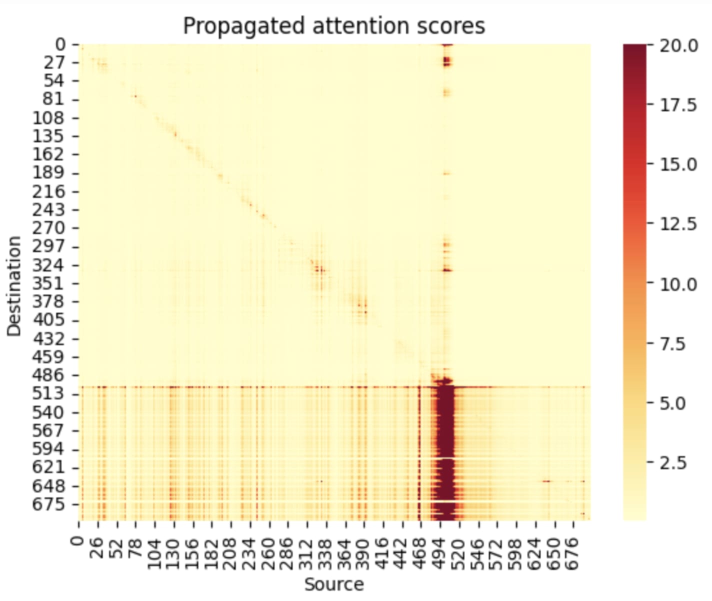
2) Encoder attention is highly localized

Interestingly, the encoder attention patterns are highly temporally localized. This contrasts with standard LLMs which often attends to source tokens based on semantic content rather than distance to the destination token.

We propagate the attention scores $R_{t}$ down the layers of the encoder as in Generic Attention-model Explainability for Interpreting Bi-Modal and Encoder-Decoder Transformers. This roughly equates to,

$R_{t + 1} = R_{t} + {¯ A}_{t + 1} R_{t},$

where,
${¯ A}_{t} = E [\nabla A_{t} \circ A_{t}],$

$A_{t}$ is the attention pattern in layer $t$ and ${¯ A}_{t}$ is the attention pattern weighted by gradient contribution. This produces the striking pattern below; up to the point where the audio ends, the attention pattern is very localized. When the speech ends (at frame ~500 in the following plot), all future positions attend back to the end of the speech.

2.2) Constraining the attention window has minimal effects on performance

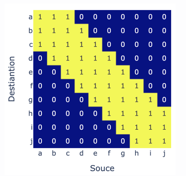
Given how localized the attention pattern appears to be, we investigate what happens if we constrain it so that every audio embedding can only attend to the k nearest tokens on either side. Eg if k=2 we would we apply the following mask to the attention scores before the softmax:

Here are the transcripts that emerge from a short audio clips from Hot Ones as we limit the attention window for various values of k. We observe that even when our attention window is reduced to k=75 (normally k=750), the model continues to generate reasonably accurate transcripts, indicating that information is being encoded in a localized manner.

Attention window size	Transcript
Original transcript (k=750)	‘hot ones. The show where celebrities answer hot questions while feeding even hotter wings.’
k=100	‘Hot ones. The show where celebrities answer hot questions, what feeding, eating hot wings. I am Shana Evans. I’m Join Today.’
k=75	‘The show with celebrities and their hot questions, what feeding, eating hot wings. Hi, I’m Shannon, and I’m joined today.’
k=50	‘The show where celebrities enter hot questions, what leading, what leading, what are we.’
k=20	‘I’m joined today’
k=10	’’

2.3) We can precisely remove words from a transcript by removing their corresponding embeddings

Recall that Whisper is an encoder-decoder transformer; the decoder cross-attends to the output of the final layer of the encoder. Given the apparent localization of the embeddings in this final layer, we postulate that we could remove words from the transcript by ‘chopping’ out their corresponding embeddings. Concretely we let,

final_layer_output[start_index:stop_index] = final_layer_output_for_padded_input[start_index:stop_index]

Consider the following example in which we substitute the initial 50 audio embeddings with padded equivalents (e.g., start_index=0, stop_index=50). These 50 embeddings represent (50/1500)*30s=1s of audio. Our observation reveals that the transcript resulting from this replacement omits the initial two words. The fact that we can do this, suggests that for each word in the transcript, the decoder is cross-attending to a small window of audio embeddings and using a limited amount of context from the rest of the audio embeddings.

Original Transcript:

`hot ones. The show where celebrities answer hot questions while feeding even hotter wings.`

Substitute embedding between (start_index=0, stop_index=50):

`The show where celebrities answer hot questions while feeding even hotter wings.`

We can also do this in the middle of the sequence. Here we let (start_index=150, stop_index=175) which corresponds to 3-3.5s in the audio and observe that the transcript omits the words `hot questions`:

Original:

`hot ones. The show where celebrities answer hot questions while feeding even hotter wings.`

Substitute embeddings between (start_index=150, stop_index=175):

`hot ones. The show where celebrities while feeding even hotter wings.`

3) The decoder alone acts as a weak LM

Whisper is trained exclusively on supervised speech-to-text data; the decoder is not pre-trained on text. In spite of this, the model still acquires rudimentary language modeling capabilities. While this outcome isn’t unexpected, the subsequent experiments that validate this phenomenon are quite interesting/amusing in themselves.

3.1) Whisper learns language modelling bigrams

If we just use ‘padding’ frames as the input of the encoder and ‘prompt’ the decoder we can recover bigram statistics. For example, at the start of transcription, the decoder is normally prompted with:
<|startoftranscript|><|en|><|transcribe|>

Instead we set the ‘prompt’ to be:
<|startoftranscript|><|en|><|transcribe|> <our_prompt_token>

This is analogous to telling the model that the first word in the transcription is <our_prompt_token>.

Below we plot the top 20 most likely next tokens and their corresponding logit for a variety of prompts. We can see that when the model has no acoustic information it relys on learnt bigrams.

3.2) Words embeddings are clustered by semantic and acoustic similarity

Bigram statistics are often learnt by the token embedding layer in transformer language models. Additionally in LLMs, we observe semantically similar words clustered in embedding space. This phenomenon also holds for Whisper, but additionally we discover that words with similar sounds also exhibit proximity in the embedding space. To illustrate this, we choose specific words and then create a plot of the 20 nearest tokens based on their cosine similarity.

‘rug’ is close in embedding space to lug, mug and tug. This is not very surprising of a speech-to-text model; if you think you hear the word ‘rug’, it is quite likely that the word was in fact lug or mug.

3.3) The decoder learns semantic features analogous to those found in LLMs

Finally, we collected maximally activating dataset examples (using the same dataset of 10,000 2s audio clips) for the neuron basis of decoder blocks.0.mlp.1. We find that they often activate on semantically similar concepts, suggesting that a) the model is already activing on the word level by the first MLP layer and b) it has aquired rudimentary language modelling capabilities like a weak LLM. Below we show the transcripts for the maximally activating dataset examples for some neurons in decoder.blocks.0.mlp.1.

Neuron 10 - Food related

Dataset example	1	2	3	4	5
Transcript	’Better food	″I’m a steak	″cheese	″on a meal.	″this salad’
Dataset example	6	7	8	9	10
Transcript	’I’ve been eating	’for lunch	″Rice	″and after dinner	″dinner’

Neuron 12 - Numbers (particularly *th)

Dataset example	1	2	3	4	5
Transcript	’than 15	″the 8th	″at 5	″ Amen Perth	″of 16th’
Dataset example	6	7	8	9	10
Transcript	’the 20th	″6th year	″Until the 6th′	3,000	′Stay at 4th’

Neuron 14 - Verbs related to moving things

Dataset example	1	2	3	4	5
Transcript	’or throw	″to knock the rear	″or shaking	″such knock	″I’ll drill you’
Dataset example	6	7	8	9
Transcript	’was brushing	″Just throw	″swept the	″to struck’

Conclusion

To the best of our knowledge, this work presents the first attempt to do interpretability on a multimodal audio-text model. We have demonstrated that acoustic features are human interpretable and formulated a way of listening to them. Additionally, we have also presented some macroscopic properties of Whisper’s encoder and decoder. Our findings reveal that the audio encoder’s attention is highly localized, in contrast to the semantically aware attention patterns observed in Large Language Models. Furthermore, despite being exclusively trained on a supervised speech-to-text task, the decoder has acquired basic language modelling capabilities. This is a first step in developing universal interpretability techniques that can be used to detect dangerous/deceptive computation in multimodal models. This work is however by no means comprehensive. A notable limitation is that we simply used dataset examples to demonstrate acoustic features (rather than using an optimization based method like DeepDream) potentially biasing features towards the dataset. Future work would include getting an optimization based feature visualization method working in the audio domain, in addition to looking more closely into how the acoustic features in the encoder are mapped to linguistic ones in the decoder.

Interpreting OpenAI’s Whisper