Toward Statistical Mechanics Of Interfaces Under Selection Pressure
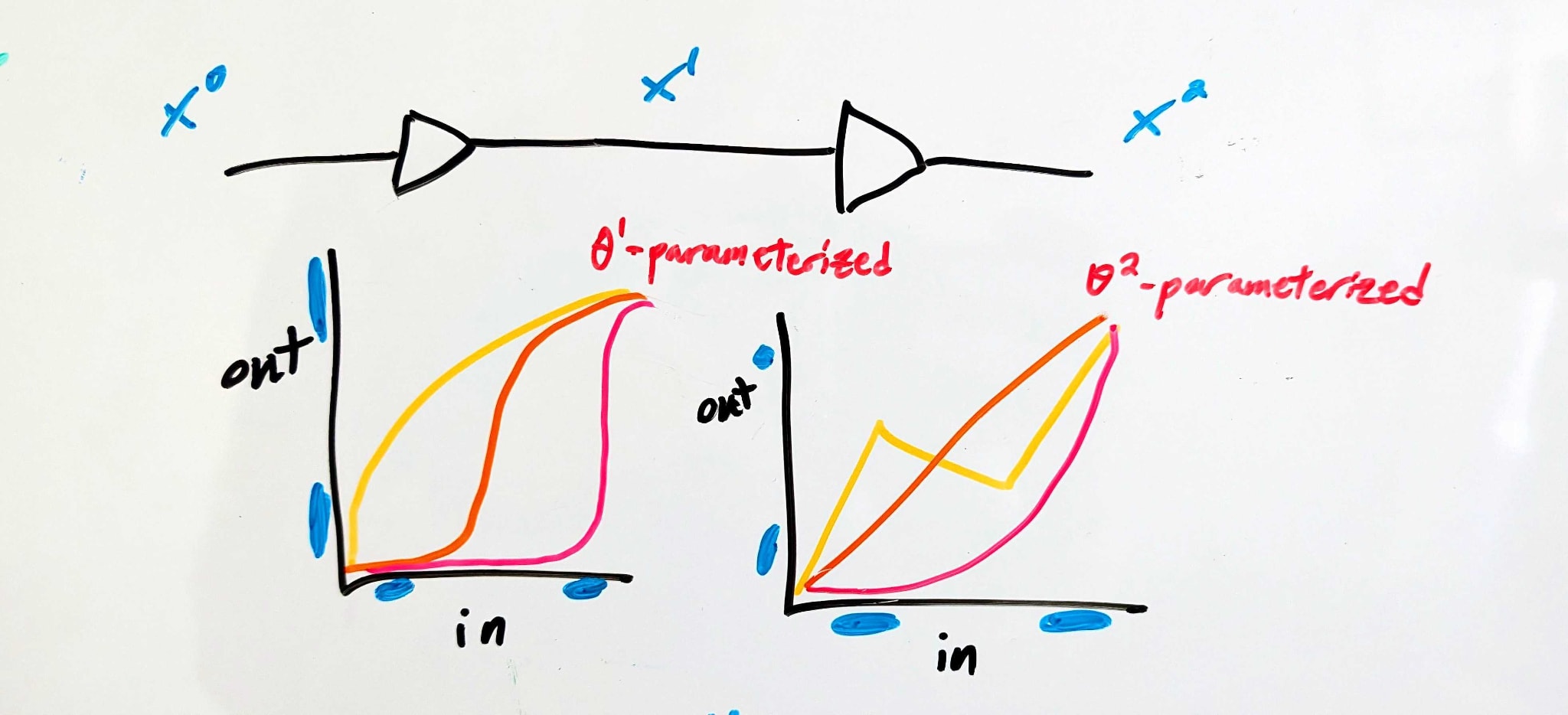
Imagine using an ML-like training process to design two simple electronic components, in series. The parameters control the function performed by the first component, and the parameters control the function performed by the second component. The whole thing is trained so that the end-to-end behavior is that of a digital identity function: voltages close to logical 1 are sent close to logical 1, voltages close to logical 0 are sent close to logical 0.

Background: Signal Buffering
We’re imagining electronic components here because, for those with some electronics background, I want to summon to mind something like this:
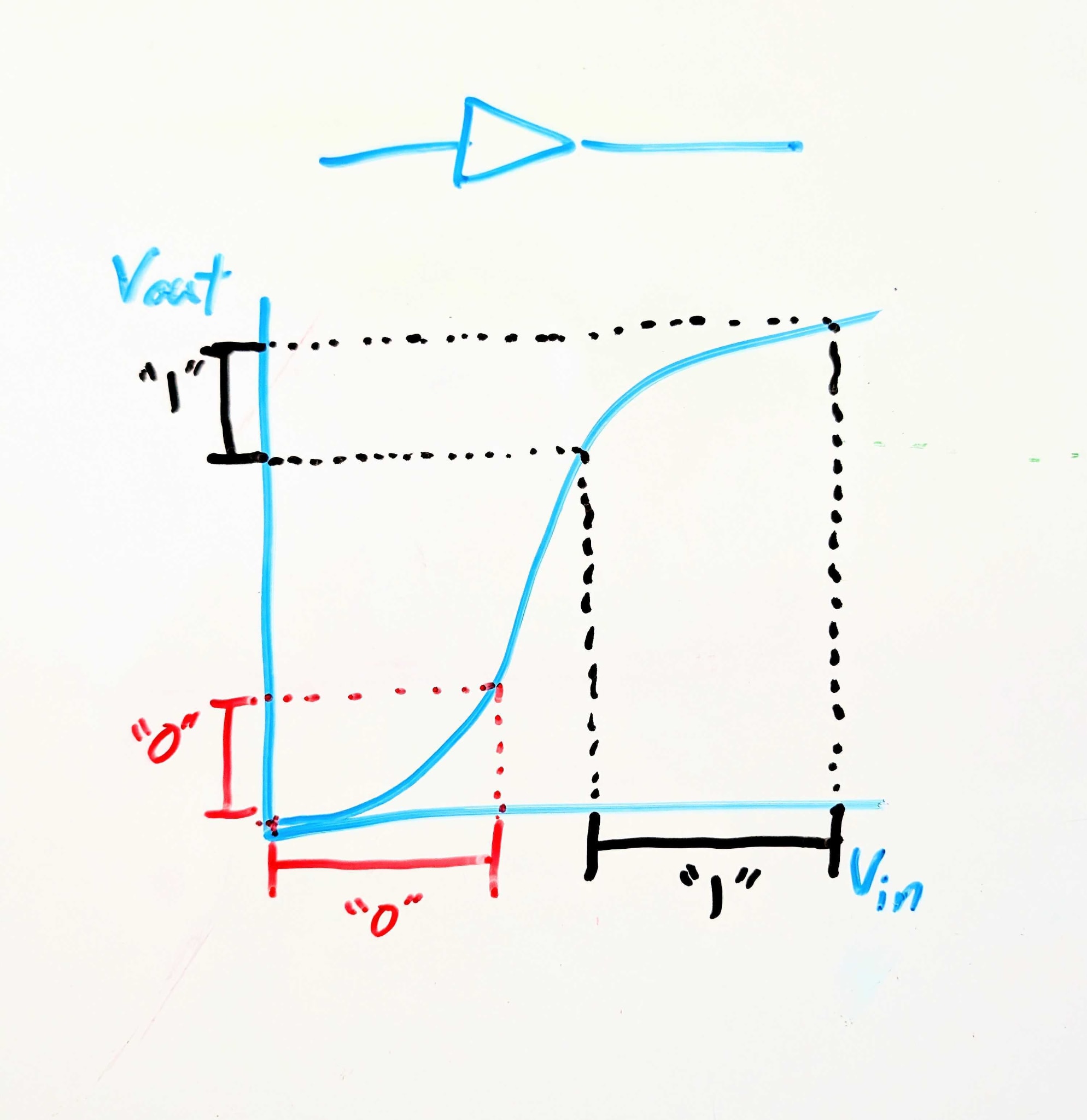
This electronic component is called a signal buffer. Logically, it’s an identity function: it maps 0 to 0 and 1 to 1. But crucially, it maps a wider range of logical-0 voltages to a narrower (and lower) range of logical-0 voltages, and correspondingly for logical-1. So if noise in the circuit upstream might make a logical-1 voltage a little too low or a logical-0 voltage a little too high, the buffer cleans that up, pushing the voltages closer to their ideal values.
This is a generalizable point about interfaces in scalable systems: for robustness and scalability, components need to accept less-precise inputs and give more-precise outputs.
That’s the background mental picture I want to invoke. But now, I want to combine it with an ML-like mental picture of training a system to match particular input/output behavior.
Back To The Original Picture: Introducing Interfaces
Here’s a conceptual story.
There are three interfaces—“APIs”, we’ll call them. The first () is at the input of the whole system, the second () between the two components, and the last () is at the output of the whole system. At each of those APIs, there’s a set of “acceptable” voltages for each logical input to the full system (i.e. 0 or 1).
The APIs constrain the behavior of each component—e.g. component 1 is constrained by (which specifies its inputs) and (which specifies its outputs).
Let’s put some math on that, with some examples.
A set of APIs might look like:
- i.e. the full system accepts either a voltage between 0 and 1.2 volts (representing logical 0), or a voltage between 3.5 and 5.0 volts (representing logical 1). No particular behavior is guaranteed for other voltages.
- i.e. in the middle the system uses extreme voltages (either above 4.6 or below 0.5 volts) to represent logical 0, and middling voltages to represent logical 1. Weird, but allowed.
- i.e. a narrower range of low voltages but wider range of high voltages, compared to the input. This might not be the most useful circuit behavior, but it’s an allowed circuit behavior.
(For simplicity, we’ll assume all voltages are between 0V and 5V). In order for the system to satisfy those particular APIs:
Component 1 must map every value in to a value in , and every value in to a value in - i.e. any value less than 1.2V must be mapped either below 0.5V or above 4.6V, while any value above 3.5V must be mapped between 2.6 and 3.8V.
Component 2 must likewise map every value in to a value in , and every value in to a value in .
Using for component and writing it out mathematically: the components satisfy a set of APIs if and only if
That’s a set of constraints on , for each component .
The Stat Mech Part
So the APIs put constraints on the components. Furthermore, subject to those constraints, the different components decouple: component 1 can use any parameters internally so long as it satisfies the API set (specifically and ), and component 2 can use any parameters internally so long as it satisfied the API set (specifically and ).
Last big piece: putting on our stat mech/singular learning theory hats, we educatedly-guess that the training process will probably end up with an API set which can be realized by many different parameter-values. A near-maximal number of parameter values, probably.
The decoupling now becomes very handy. Let’s use the notation - you can think of it as the log number of parameter values compatible with the constraints, or as entropy or relative entropy of parameters given constraints (if we want to weight parameter values by some prior distribution, rather than uniformly). Because of the decoupling, we can write H as
So there’s one term which depends only on component 1 and the two APIs adjacent to component 1, and another term which depends only on component 2 and the two APIs adjacent to component 2.
Our stat-mech-ish prediction is then that the training process will end up with a set of APIs for which is (approximately) maximal.
Why Is This Interesting?
What we like about this mental model is that it bridges the gap between stat mech/singular learning theory flavored intuitions (i.e. training finds structure compatible with the most parameters, subject to constraints) and internal structures in the net (i.e. internal interfaces). This feels to us like exactly the gap which needs to be crossed in order for stat mech flavored tools to start saying big things about interpretability.
When you say that the training process ends up with an API set, do you mean that instead of the usual order where you prescribe constraints for the training process to move around in, which you enforce e.g. by clipping the parameters to the nearest values that satisfy the constraints after each training step, you start with any training process and then use constraints to describe its behavior?
e.g. for n bodies with approximately-known initial positions and velocities, subject to gravity, we may be unable to predict precisely where the bodies end up, but we can potentially use energy conservation to put bounds on the coordinates they can ever reach, and if we keep listing out provable constraints, we are eventually left unable to predict any further details of the system?
Yes.
Problem with this: I think training tasks in real life are usually not, in fact, compatible with very many parameter settings. Unless the training task is very easy compared to the size of the model, basically all spare capacity in the model parameters will be used up eventually, because there’s never enough of it. The net can always use more, to make the loss go down a tiny bit further, predict internet text and sensory data just a tiny bit better, score a tiny bit higher on the RL reward function. If nothing else, spare capacity can always be used to memorise some more training data points.H(Θ|API) may be maximal given the constraints, but the constraints will get tighter and tighter as training goes on and the amount of coherent structure in the net grows, until approximately every free bit is used up.[1]
But we can still ask whether there are subsets of the training data on which the model outputs can be realised by many different parameter settings, and try to identify internal structure in the net that way, looking for parts of the parameters that are often free. If a circuit stores the fact that the Eiffel tower is in Paris, the parameter settings in that circuit will be free to vary on most inputs the net might receive, because most inputs don’t actually require the net to know that the Eiffel tower is in Paris to compute its output.
A mind may have many skills and know many facts, but only a small subset of these skills and facts will be necessary for the mind to operate at any particular moment in its computation. This induces patterns in which parts of the mind’s physical implementation are or aren’t free to vary in any given chunk of computational time, which we can then use to find the mind’s skills and stored facts inside its physical instantiation.
So, instead of doing stat mech to the loss landscape averaged over the training data, we can do stat mech to the loss landscapes, plural, at every training datapoint.
Some degrees of freedom will be untouched because they’re baked into the architecture, like the scale freedom of ReLU functions. But those are a small minority and also not useful for identifying the structure of the learned algorithms. Precisely because they are guaranteed to stay free no matter what algorithms are learned, they cannot contain any information about them.
A successfully trained 1 hidden layer perceptron with 500 hidden activations has at absolute minimum 500! possible successful parameter settings.
See footnote. Since this permutation freedom always exists no matter what the learned algorithm is, it can’t tell us anything about the learned algorithm.
I like this! Nice useful mental model.
NB: the notion of an interface is connected to formal verification: in order to formally verify a neural network, you have to provide a proof / certificate that the model really does adhere to an interface; for every possible value in the input domain, it outputs a value in the output domain.
Seems like the main additional source of complexity is that each interface has its own local constraint, and the local constraints are coupled with each other (but lower-dimensional than parameters themselves); whereas regular statmech usually have subsystems sharing the same global constraints (different parts of a room of ideal gas are independent given the same pressure/temperature etc)
To recover the regular statmech picture, suppose that the local constraints have some shared/redundant information with each other: Ideally we’d like to isolate that redundant/shared information into a global constraint that all interfaces has access to, and we’d want the interfaces to be independent given the global constraint. For that we need something like relational completeness, where indexical information is encoded within the interfaces themselves, while the global constraint is shared across interfaces.