Neural Networks learn Bloom Filters
Overview:
We train a tiny ReLU network to output sparse top-
Here’s what a small network trained on a toy version of the sparse top-
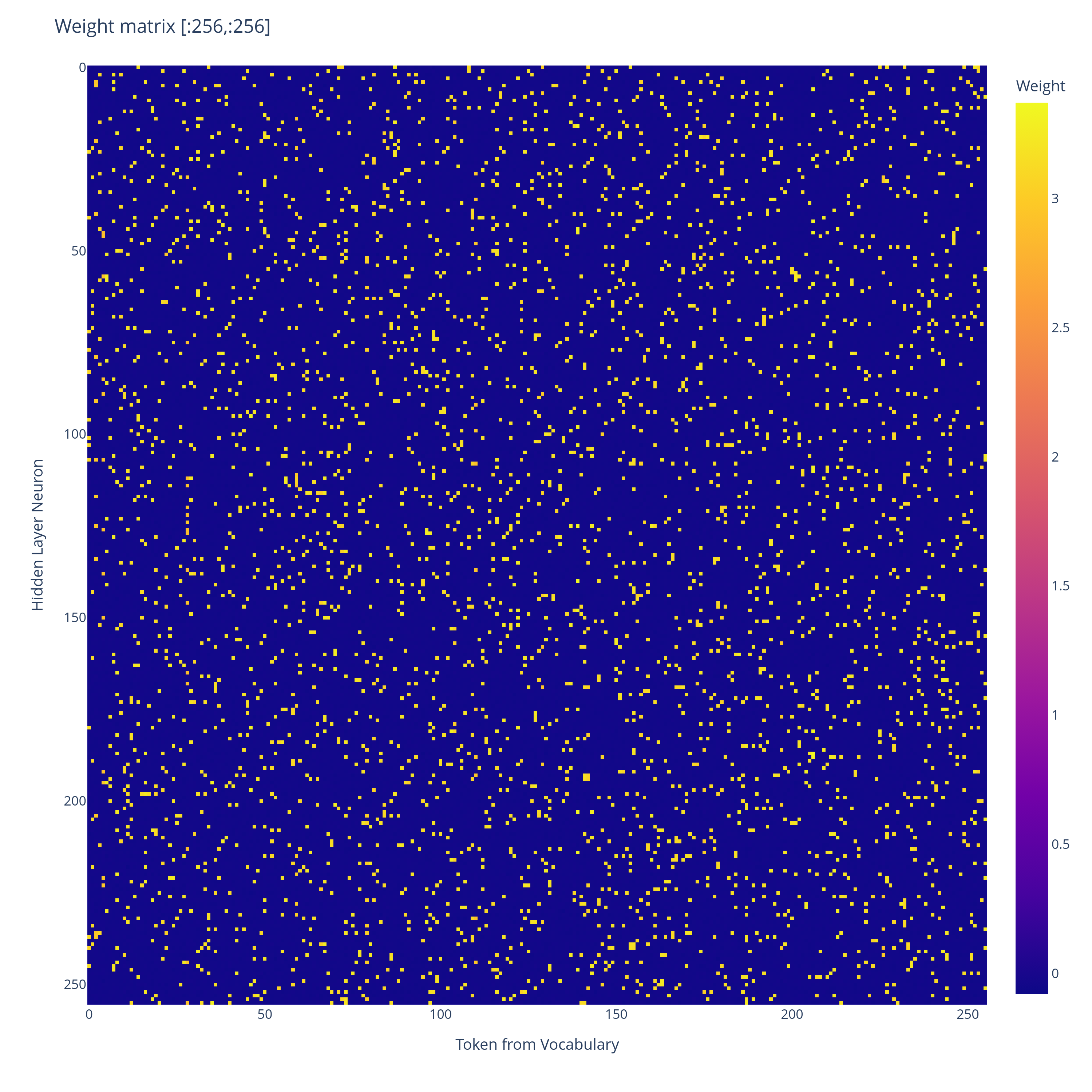
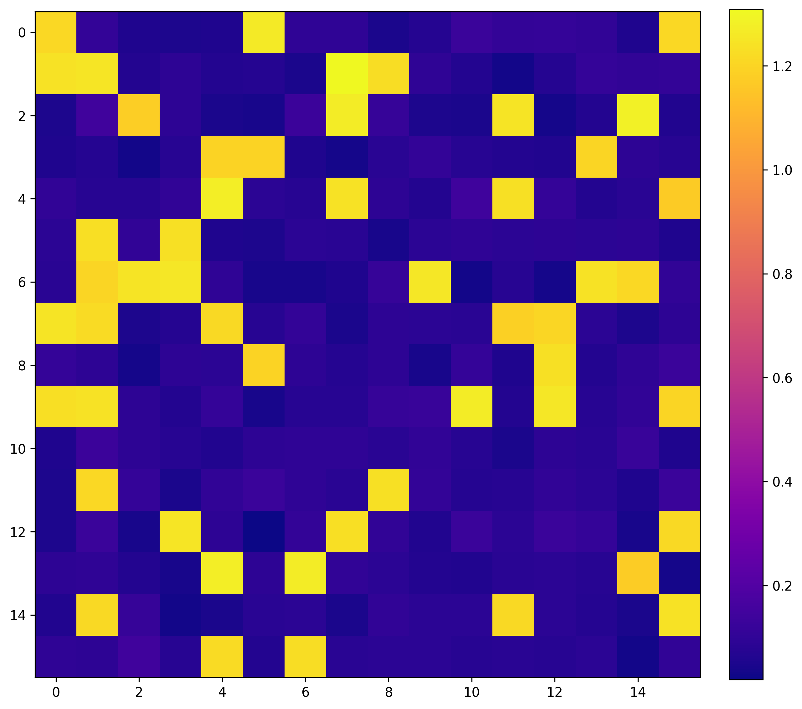
Weight matrix
Plot of the range of values of
That’s the input weight matrix of the trained network. Every entry is either
We provide a theoretical construction showing how to set the weights to exactly implement a Bloom filter. The real network seems to learn to do something similar, and seems to behaviourally act like a Bloom filter, but while we provide a fair bit of mechanistic evidence, we don’t yet have a complete mechanistic explanation of the trained network.
Additionally, this is just a toy network, so it doesn’t directly tell us about what larger models might do. But I found the discreteness of the learned algorithm to be very interesting.
It seems to learn a probabilistic solution which scales like
The Task:
As a result of reading The Softmax Bottleneck, I have gotten quite interested in what mechanisms toy MLP networks learn to output sparse probability distributions. I have tried to devise a toy problem to address this question.
We sample token indices
We give as input to a
Let
The task is to minimise the expected KL divergence between
We vary
Construction:
The construction below is my hypothesis for what the
I had Claude prepare an animation to visualise the construction.
The initial residual stream is given as a weighted sum of the hashes of the top-
The discreteness of the logits allows exactly uniform probability to be assigned to the top-
Formal construction:
We use a
Fix
For each
For each
Set
Set
Analysis of a single forward pass:
The residual stream initially is given by an input vector
By construction, the
Then the final residual stream is given by
So we want to have with high probability over uniform random choice of
This is precisely the same situation as that of a Bloom filter (Youtube video that explains them better than I could), also see the wikipedia article.
The standard bloom filter analysis applies and we get scaling of
Interestingly the false positive case just looks like another token being included in the top-
Training:
I trained a
The model used vocabulary size
For each training example, a uniformly random subset of
The network was trained for
The final model achieved total variation distance
Behavioural analysis of the trained network:
We draw sets of tokens uniformly without replacement from
Probability mass assigned to the top-
PDF of probability assigned to the top-
So we have a distinct rarely occurring cluster where the top-
A typical top-
Distribution of top-
After
Distribution of top-
You can see how the network fairly robustly handles the false positive. It doesn’t significantly disrupt the top-
Interestingly, we can also provide
Conditioning on there being even a single false positive, we expect the union of hashes to be large, which means we should expect other tokens to have large intersection with the union. We see this in the above figure, with significant probability mass going to tokens
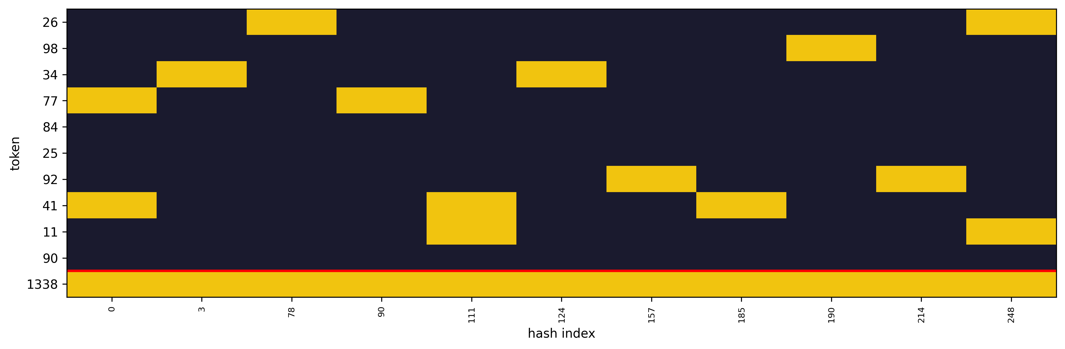
The hash of token
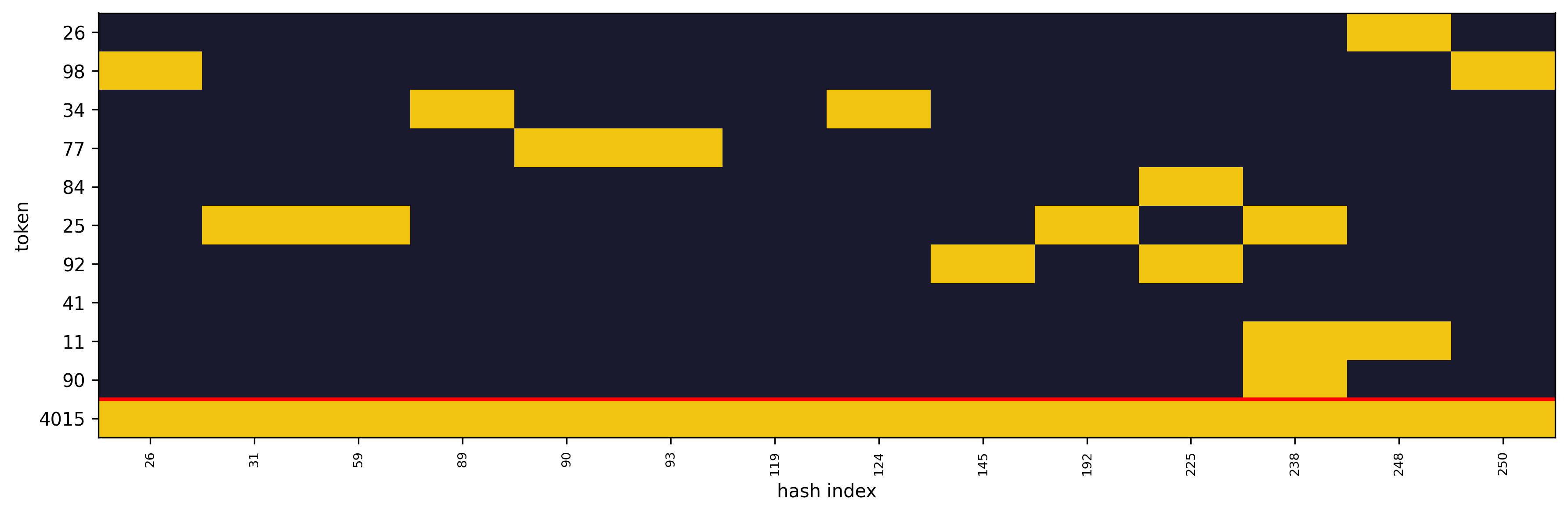
The hash of token
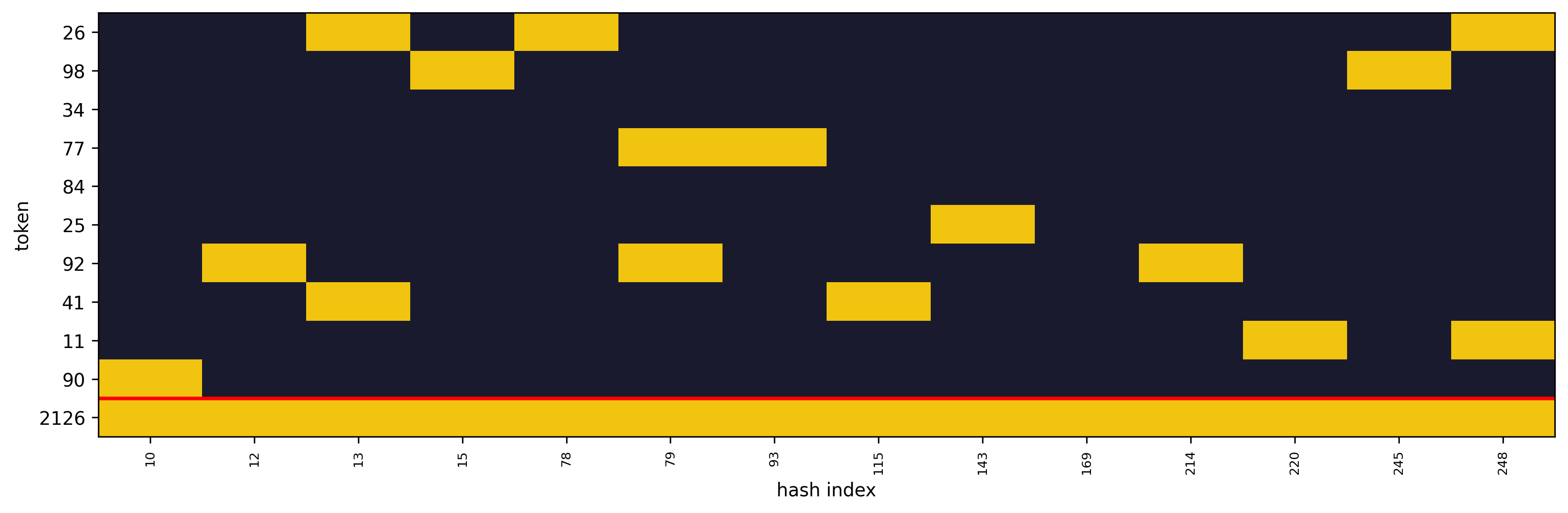
Ditto for token
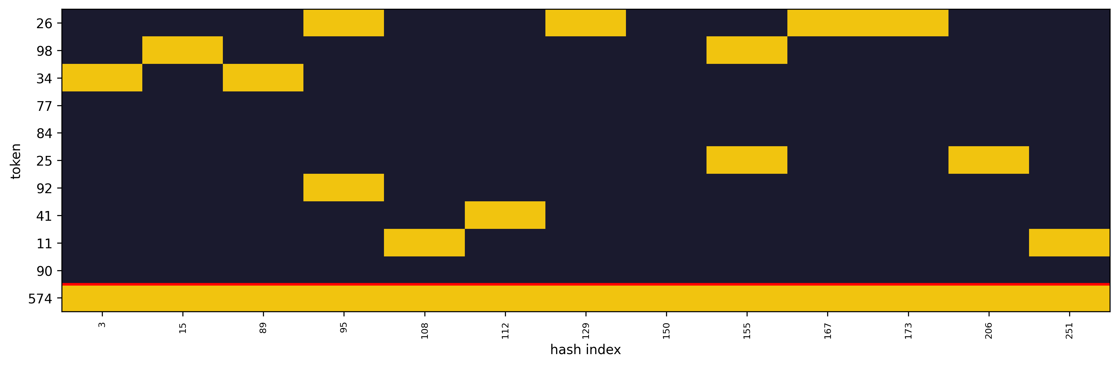
Token
As a baseline, here is Token
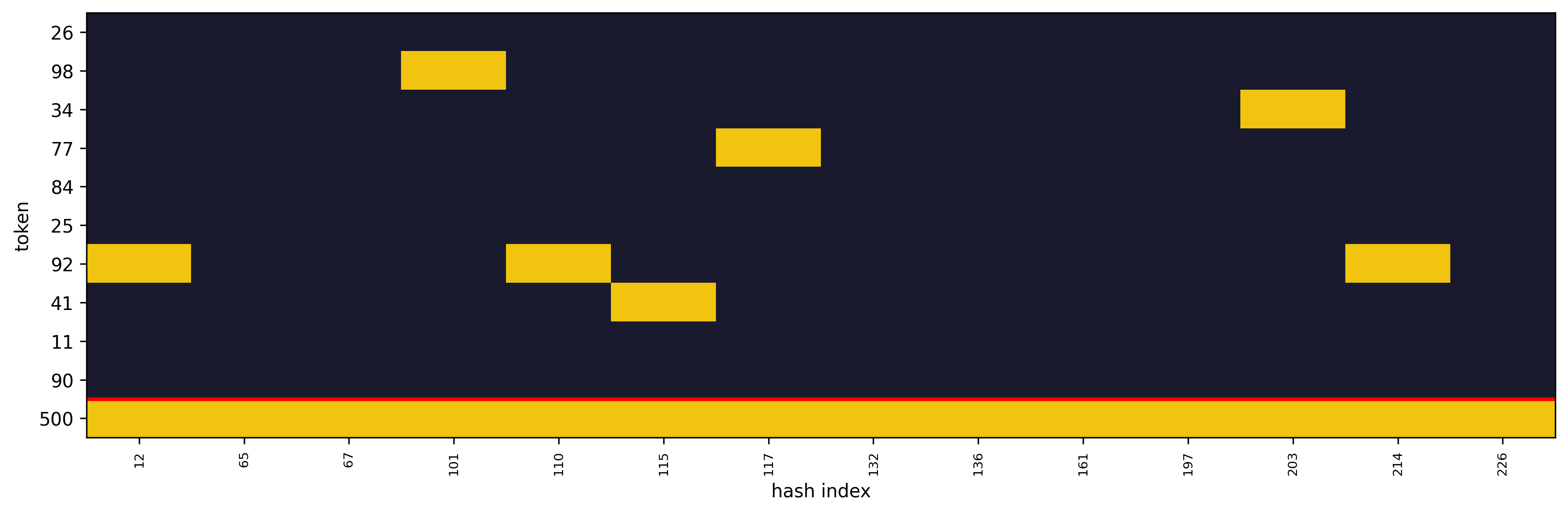
In a
Mechanistic analysis of the trained network:
Now we have seen that the model seems to behave like a Bloom filter, we give a partial mechanistic analysis of how the trained weights help to implement the filter.
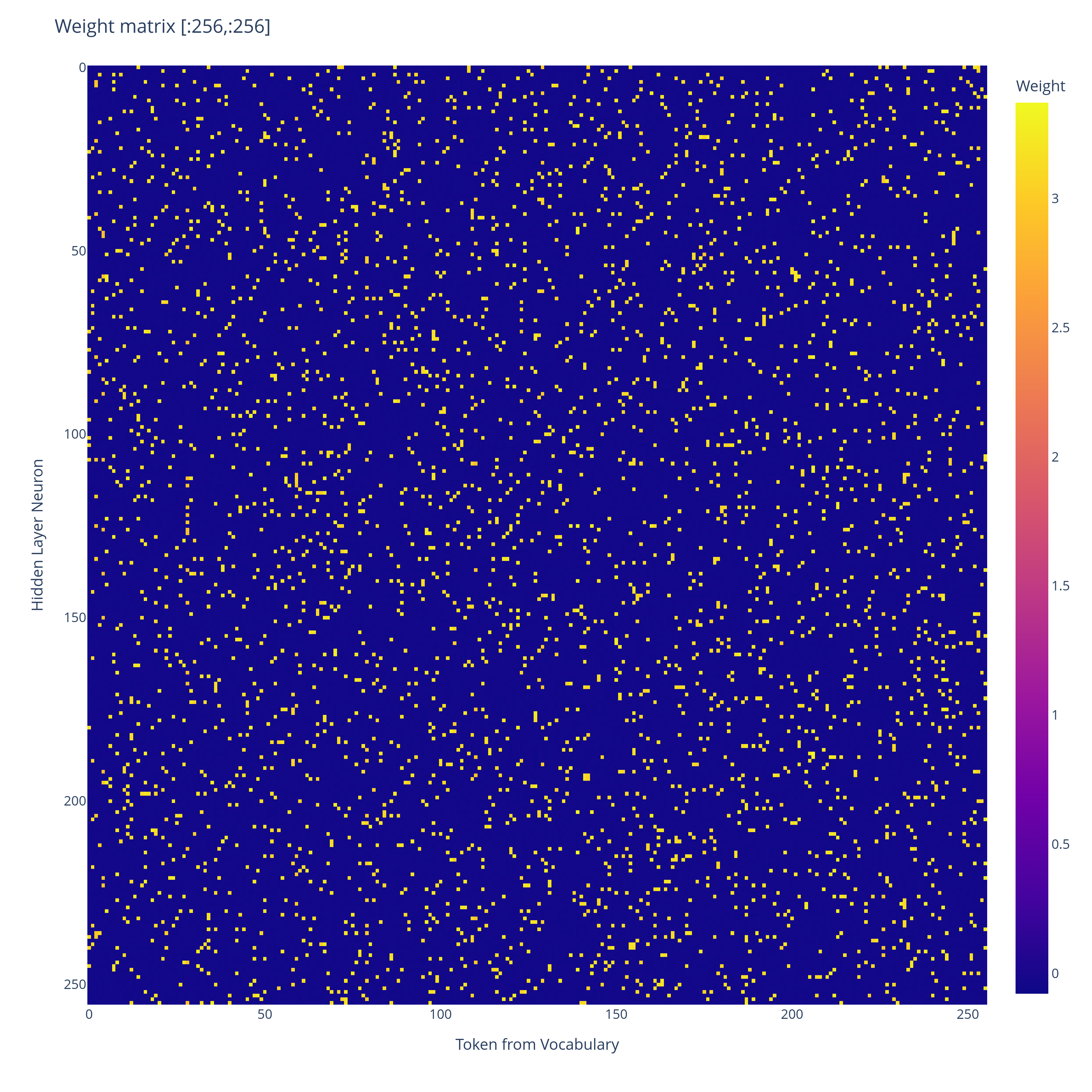
Learned
Distribution of values in
The fact that the positive values vary in magnitude (in contrast to our construction, which uses a constant value
Learned
Distribution of values in
Since both
Perfect match between the transpose of one mask and the other mask.
So
To connect with our mechanistic story further, we linearly transform the residual stream
If the trained network were acting as our construction expects it to, then
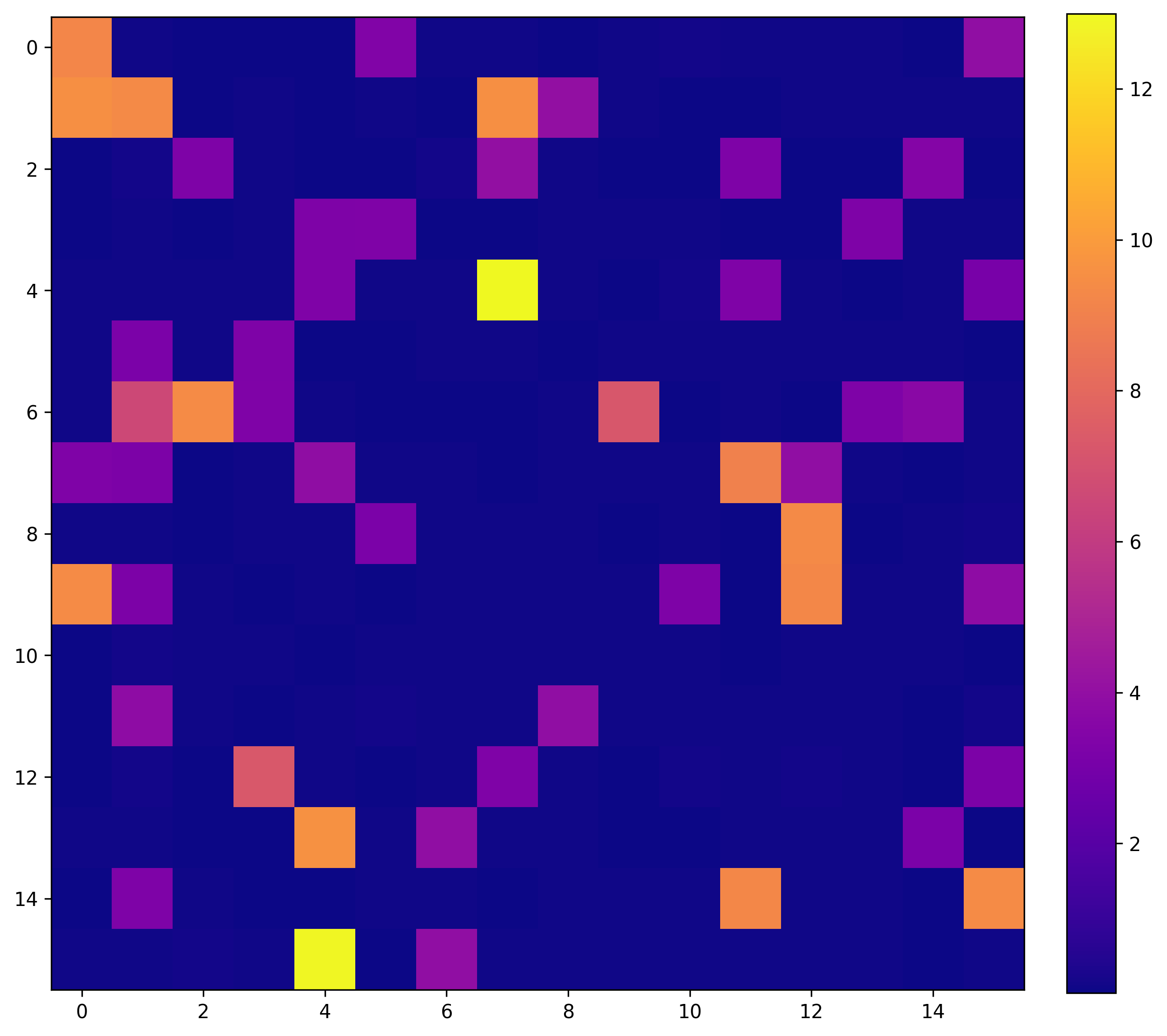
Distribution of values of
For this input, a value is dark blue iff it doesn’t belong to the union of the “hashes” (as given by the mask of
Note that, just as in Claude’s animation, among the dimensions contained in the union of the hashes, there is a wide range of possible values that are taken on. We have values ranging from
There are discrete clusters in the distribution of values, which seems to correspond to the number of intersecting hashes at each position.
The job of the hidden layer seems to be to collapse this range in values to produce an indicator of the union of hashes.
This corresponds to the second residual stream in Claude’s animation.
Distribution of values of
The hash values which in the initial residual stream were significantly above the others have been clamped, and the union of the hashes now lies in a fairly narrow range.
To get from
There can be a wide variance in the raw values of the hash containing matrix
Values of
The above is the dot product of the large positive terms in the
Nonetheless, since there is a gap of about
We aren’t fine grained enough to argue why we get so close to a uniform distribution over the top-
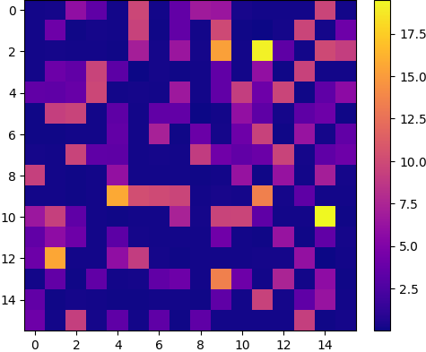
What’s interesting about the above figure is that it’s pathological because the union of hashes is large. The union of the hashes being large means that it’s more likely for the hashes of non top-
But the way that you get a large union of hashes is by having top-
Which is the opposite intuition from usual, where we want to minimise interference between features!
Conclusion / Reflections:
I find multiple things interesting about the solution to the task:
In contrast to other approaches that have been discussed for neural networks handling many more features than they have dimensions in the residual stream, the solution does not rely on with 100% probability having a bounded amount of error
The scaling is a lot better behaved with this probabilistic approach. We get
Because of the form of our solution to the task, the harder task of specifying an arbitrary conditional distribution over the top-
It’s always been a bit of a mystery to me how LLMs like GPT-2 with
More broadly, i’m working on probabilistic methods for performing computation in superposition. This was a fun toy case I found for showcasing the advantages of using a probabilistic approach. I view the result on
Related work:
Prior work—The Softmax Bottleneck Does Not Limit the Probabilities of the Most Likely Tokens—shows that with
They find
I don’t think it’s mechanistically plausible that trained networks actually learn to find the
Further work:
Is it possible to fully understand the mechanism behind the
What is the scaling for the density of the hashes that the model learns? How does this relate to theoretical Bloom filter density?
What mechanisms do real LLMs learn to output distributions? Modern LLMs increasingly have
I have not read this properly yet, but at a glance this looks good to me, and I would like there to be more of this kind of thing.