AISC team report: Soft-optimization, Bayes and Goodhart

This is a report on our work in AISC Virtual 2023.

For AISC 2023, our team looked into the foundations of soft optimization. Our goal at the beginning was to investigate variations of the original quantilizer algorithm, in particular by following intuitions that uncertainty about goals can motivate soft optimization. We ended up spending most of the time discussing the foundations and philosophy of agents, and exploring toy examples of Goodhart’s curse.

Our discussions centered on the form of knowledge about the utility function that an agent must have, such that expected utility maximization isn’t the correct procedure (from the designer’s perspective). With well-calibrated beliefs about the true utility function, it’s always optimal to do Expected Utility maximization. However, there are situations where an agent is very sensitive to prior specification, and getting this wrong can have a large impact on the true utility achieved by the agent. Several other unrelated threads were pursued, such as an algorithm with high probability of above-threshold utility, and the relationship between SGD and soft optimization.

The Bayesian view on Goodhart’s law

Goodhart’s Law states that when maximizing an approximation of a true utility function, which we call proxy utility function, this leads to outcomes that are much less valuable than predicted by the proxy utility function. There is a Bayesian perspective from which it doesn’t look like Goodhart’s law will be a problem at all, namely if the agent has correct beliefs about the quality of the approximation. An ideal rational agent would represent the information they have about the world with a probability distribution that they arrived at by Bayesian reasoning. We assume that they represent their goals as a utility function over world states or as a belief distribution over such utility functions. Thus, they select actions by maximizing the expected utility over goals and world models.

If the agent was able to perfectly capture all available information about goals into an “ideal”^[1] belief distribution, maximizing the utility in expectation over this distribution would be optimal.^[2] It would avoid Goodhart’s law as much as possible given the agent’s knowledge by anticipating any overestimation of the true utility function by the proxy utility function. In this section, we try to formalize this intuition. Sadly, Bayesian reasoning is intractable in practice, both because specifying the prior is difficult and because updating the distribution is computationally hard. This framing is explained in more detail in Does Bayes Beat Goodhart?.^[3]

Beliefs about values are difficult to deal with, because you may not have a reliable way to update these beliefs after deployment. In this situation the agent’s behavior is heavily dependent on the way we specify the priors.

Setup and notation

We generally consider situations where an agent can choose a single action $a\in A$ from some space $A$. For that choice, we are interested in knowledge about the (true) utility function $v:A\to R$, $a\mapsto v\left(a\right)$ that we want the agent to maximize. The situation might include observed variables $Obs$ and hidden variables $h$. The agent models each of them respectively by random variables $V$, $\text{Obs}$ and $H$. We denote the ideal prior belief distribution, without prior misspecification or compute limitation, by $\varphi (V,\text{Obs},H)$. We denote the belief distribution that the agent estimated by $\tilde{\varphi }(V,\text{Obs},H)$.^[4] Hidden variables are used in some of our toy examples to provide better intuition about the problem. The observed variables $\text{Obs}$ could for example be a dataset such as that containing human preferences used to train the reward model in RLHF. But in this post the observed variable is always a proxy utility function $\text{Obs}=U$. We write $E:=U-V$ for the “error” random variable that indicates the error between the proxy utility and true utility functions.

Goodhart’s law

Goodhart’s law can be formalized in different ways; here we focus on “regressional Goodhart”. We will model the situation where the difference between the true and proxy utilities for a given action $a$ is given by an error term $E\left(a\right)$:

$U\left(a\right)=V\left(a\right)+E\left(a\right)$

We will now assume that the proxy utility function is an unbiased estimator of the true utility function, i.e. $E_{\varphi (U|V=v)}U=v$, or equivalently that the error function is the zero function in expectation, i.e. $E_{\varphi (E|V=v)}E=0$.

In expectation over $\varphi \left(V\right)$ and evaluated at any action $a\in A$, this yields

$E_{\varphi (V,U)}\underset{\text{estimate of}V\left(a\right)}{\underset{}{U\left(a\right)}}=E_{\varphi \left(V\right)}V\left(a\right)=E_{\varphi (V,U)}V\left(a\right)$.

However, this equality is not true if the fixed action $a$ is replaced with the action $A^{\star }$ that optimizes $U$, that is $A^{\star }=\arg {max}_{a\in A}U\left(a\right)$. Note here that $A^{\star }$ is itself now a random variable.

N​ow, we find that

$E_{\varphi \left(V\right)\varphi \left(U|V\right)}\underset{\text{estimate of}V\left(A^{\star }\right)}{\underset{}{U\left(A^{\star }\right)}}\ge E_{\varphi \left(V\right)\varphi \left(U|V\right)}V\left(A^{\star }\right)$

and the inequality is strict under mild assumptions^[5], e.g. in all of our toy examples. Intuitively, $A^{\star }$ selects for positive error $E=U-V$ so that $E\left(A^{\star }\right)=U\left(A^{\star }\right)-V\left(A^{\star }\right)$ is positive in expectation.

So, the expected value $E_{\varphi \left(V\right)\varphi \left(U|V\right)}V\left(A^{\star }\right)$ of the action selected by proxy maximization is lower than the proxy prediction $E_{\varphi \left(V\right)\varphi \left(U|V\right)}U\left(A^{\star }\right)$, even though we assumed that U was an unbiased estimator. This is one way of stating the regressional variant of Goodhart’s law.

How Bayes could beat Goodhart

From a Bayesian perspective, the situation after observing the proxy utility function $U$ is best described by the conditional distribution $\varphi \left(V|U=u\right)$. We will therefore look at the conditional expected true utility and write it as $f(u,a)=E_{\varphi \left(V|U=u\right)}V\left(a\right)$.

The Bayes-optimal action for belief $\varphi$ is $A_{Bayes}^{\star }\left(u\right)=\arg {max}_{a\in A}f(u,a)$. While $A^{\star }$ maximizes the proxy utility $U$, $A_{Bayes}^{\star }$ maximizes the conditional expected true utility $f(U,a)$.

Just as is the case for $U$, this maximization objective also has the same expectation over $\varphi (V,U)$, as the true utility function $V$. We can see this for any action $a\in A$ as follows:

$E_{\varphi (V,U)}\underset{\text{estimate of}V\left(a\right)}{\underset{}{f(U,a)}}=E_{\varphi (V,U)}{E}_{\varphi \left(V^{\prime }|U\right)}{V}^{\prime }\left(a\right)=E_{\varphi \left(U\right)}{E}_{\varphi \left(V^{\prime }|U\right)}{V}^{\prime }\left(a\right)=E_{\varphi (V,U)}V\left(a\right)\text{.}$

But, in contrast to $U$, this equation also holds for the optimal action $A_{Bayes}^{\star }$:

$E_{\varphi (V,U)}\underset{\text{estimate of}V\left(A_{\text{Bayes}}^{\star }\right)}{\underset{}{f(U,A_{\text{Bayes}}^{\star })}}=E_{\varphi (V,U)}{E}_{\varphi \left(V^{\prime }|U\right)}{V}^{\prime }\left(A_{\text{Bayes}}^{\star }\right)=E_{\varphi (V,U)}V\left(A_{\text{Bayes}}^{\star }\right)\text{.}$

Intuitively, this is due to the fact that the distribution $\varphi \left(V|U\right)$ used in the Bayesian maximization objective, which we used as approximation of $V$, is the same as the distribution from which $V$ is indeed sampled (at least according to the agent’s best knowledge).

In this sense, “Bayes beats Goodhart”. The Bayesian maximization objective $E_{\varphi \left(V|Obs\right)}V$ does not have the problem that by maximizing it, it ceases to be a good approximation of the true utility function $V$. As a consequence, the Bayesian maximization objective also doesn’t suffer from Goodhart’s law.

As a consequence of stochasticity in the belief distribution $\varphi \left(V|U\right)$, the selected action might still turn out to perform poorly according to V, but it was the best the agent could have selected with its knowledge.

Why Bayes can’t beat Goodhart

However, we think that in practice an agent would not be able to access the ideal belief distribution $\varphi$. This is firstly because specifying priors is notoriously difficult, and because optimal actions usually require pushing away from regions of action-space where we (the designers) have a lot of data about the true value, so an agent is always heavily reliant on prior information about the reliability of the proxy. And secondly, computational limitations might mean that the distribution $\varphi \left(V|U\right)$ can’t be computed exactly.

See Abram Demski’s post, Does Bayes Beat Goodhart?, for a more detailed discussion. We found that this topic was difficult to think about, and very philosophical.

Our best guess is that the prior has to capture all the meta-knowledge that is known to the designer, for instance about boundaries in action-space or outcome-space where there is a possibility of breaking the relationship between your proxy value and true value. One extreme example of such knowledge is deontological rules like “don’t kill people”. We are confused about exactly what are the desiderata for such a “correct” prior specification.

We explored examples related to this below, but don’t feel like we have resolved our confusion completely yet. In the next sections we look at different types of concrete examples both with and without “objectively correct” beliefs.

What if the agent can access the ideal belief distribution?

In this section, we consider the scenario of an agent that is able to represent its beliefs about the true values and the errors of the proxy variable with an ideal belief distribution. We worked through several examples, some more general and some more specific, to get a better intuition about when and why regressional Goodhart can cause the most damage, and how the Bayesian approach fares.

The recent post When is Goodhart catastrophic? by Drake Thomas and Thomas Kwa contains an in-depth analysis of a similar scenario with emphasis on how errors are distributed in heavy-tailed vs light-tailed distributions.

The scenario

For various actions, we observe the proxy values $u\left(a\right)$. Our goal is to use this information to choose the action with the highest expected value of $V\left(a\right)$. We will now assume that we know the prior distribution of the true values and the distribution of the error term, and that they are independent for each action.

By Bayes’ theorem, we can calculate then the distribution of $V\left(a\right)$ given an observed value $u$, using $P\left[U\right(a)=u\mid V(a)=v]=P\left[E\right(a)=u-v]$:

$P\left[V\right(a)=v\mid U(a)=u]=\frac{P\left[V\right(a)=v]P\left[E\right(a)=u-v]}{\int d{v}^{\prime }P\left[V\right(a)=v^{\prime }]P\left[E\right(a)=u-v^{\prime }]}.$

Given this distribution, it is now possible to calculate the expected value $E\left[V\right(a)\mid U(a)=u]$ and use this value to compare policies instead of the naive method of optimizing the proxy $U\left(a\right)$. In other words, the rational choice of the action is

$a^{\ast }=\arg {max}_{a\in A}E\left[V\right(a)\mid U(a)=u(a\left)\right]\text{.}$

Example: Generalized normal distributions

Here, we assume that both the true values as well as the error term are distributed according to the generalized normal distribution with standard deviation $\sigma =1$. The shape parameter $\beta$ of these distribution determines their “tailedness”; distributions with a smaller shape parameter have a heavier tail. We vary the shape parameters of both the error and the true value distribution and calculate the expected true value conditional on the proxy value, $E\left[V\right(a)\mid U(a)=u(a\left)\right]$, using numerical integration. The plots show the expected conditional values as a function of $u$ as well as the identity function for comparison as a dashed line.

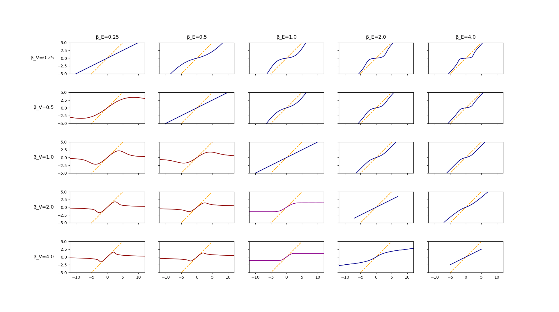
Only in the case where ${\beta }_V>{\beta }_E$ and ${\beta }_E\le 1$ do we observe that the expected value graph does not go to infinity for large values of the proxy value. That is, only in these cases to we observe Goodhart’s curse. This seems to be in agreement with the result proven in Catastrophic Regressional Goodhart: Appendix.

Example: Normally distributed error term with randomly drawn standard deviations

We wanted a concrete example where the error distribution had a free parameter that controls the variance, which we can think of as being upon observing the proxy value, which intuitively should create a situation where maximizing the proxy reduces the correlation. In this example, we assume the error is normally distributed with mean 0, but for each action the standard deviation itself is randomly drawn from an exponential distribution with rate parameter $\lambda =0.3$. For concreteness, the error values can be sampled using the following Python code:

def create_error_vector(n):
    std_dev = np.random.exponential(0.3, size=n)
    return np.random.normal(0, std_dev, size=n)

The resulting distribution of the error term can be calculated as

$\begin{array}{cc}P\left[E\right(a)=x]& ={\int }_0^{\infty }P\left[E\right(a)=x|\sigma (a)=s]P\left[\sigma \right(a)=s]ds\\ & =\frac{0.3}{\sqrt{2\pi }}{\int }_0^{\infty }\exp [-\frac{1}{2}{\left(\frac{x}{s}\right)}^2-0.3s]ds\end{array}$

We will now look at two cases for the distribution of the true values.

In the first case, we assume that the prior values are uniformly distributed in the interval [-0.5, 0.5]. Here, the graph of the expected true values look like this:

In the second case, we assume a standard Gaussian distribution (i.e. with mean $\mu =0$ and standard deviation $\sigma =1$). The graph of the expected true values looks very similar:

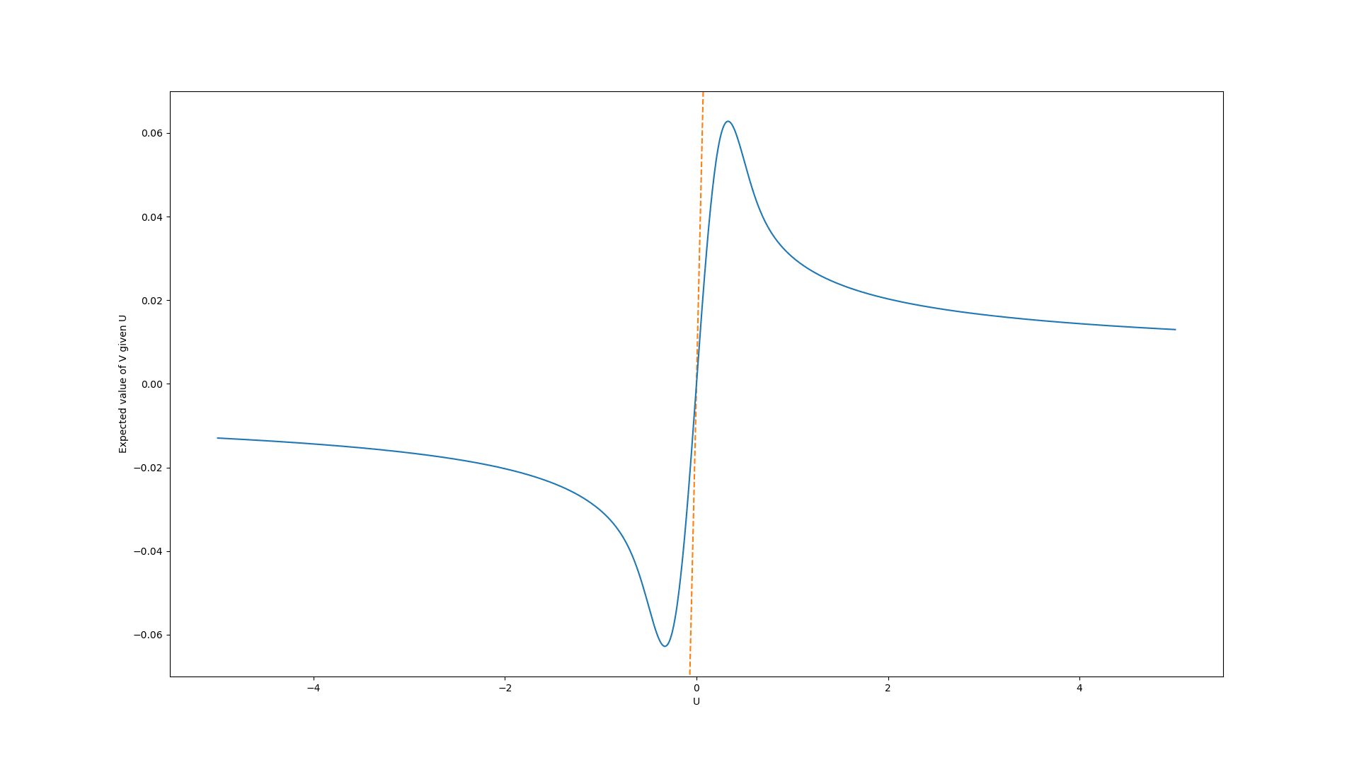
In both cases, it is clearly not optimal to choose the policies with the largest proxy values. Instead, values quite close to $u=0$ have much higher expected value and the expected value decays towards $0$ (the mean of the prior distribution) for very high values.

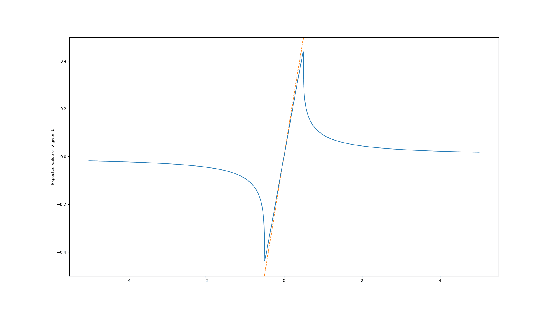
Example: Laplace-distributed error term with randomly drawn scale parameters

In this example, we assume the error is Laplace-distributed with mean $0$ and scale parameter $0.9$, but the error is “stretched” by multiplying it with a random value from an exponential distribution (with rate parameter $1$) taken to the power of $6$. This was done in an attempt to make the Goodhart effect much stronger. In other words, the error values can be sampled using the following Python code:

def create_error_vector(n):
    scale_factor = np.random.exponential(1, size=n) ** 6
    return np.random.laplace(0, 0.9 * scale_factor, size=n)

The resulting distribution can be calculated similarly to the previous example.^[6]

We again calculated the resulting graph of the expected true values for the case of a uniform and a Gaussian distribution of the error term (both with the same parameters as before).

Uniform value distribution

Gaussian value distribution

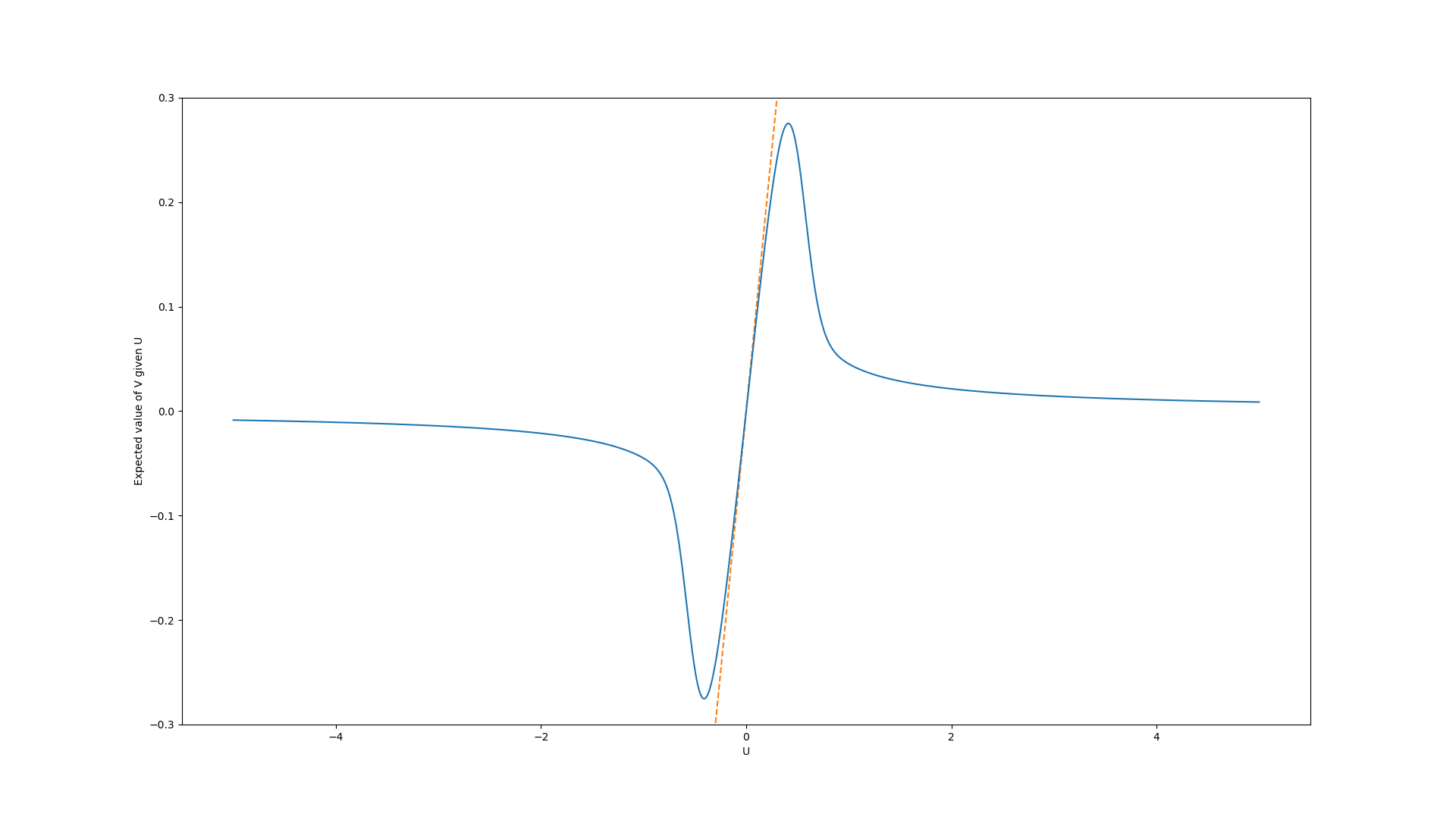
Example: Goodhart’s rollercoaster

A fun phenomenon occurs when the distribution of the error term has multiple modes. Here we combined three heavy-tailed distributions and generated the error values using the code:

def create_error_vector(n):
	locations = np.random.choice([-1, 0, 1], size = n)
	return scipy.stats.gennorm.rvs(beta = 0.25, scale = 0.0001, loc = locations)

Combined with uniformly-distributed true values, this results in an expected true value graph like this:

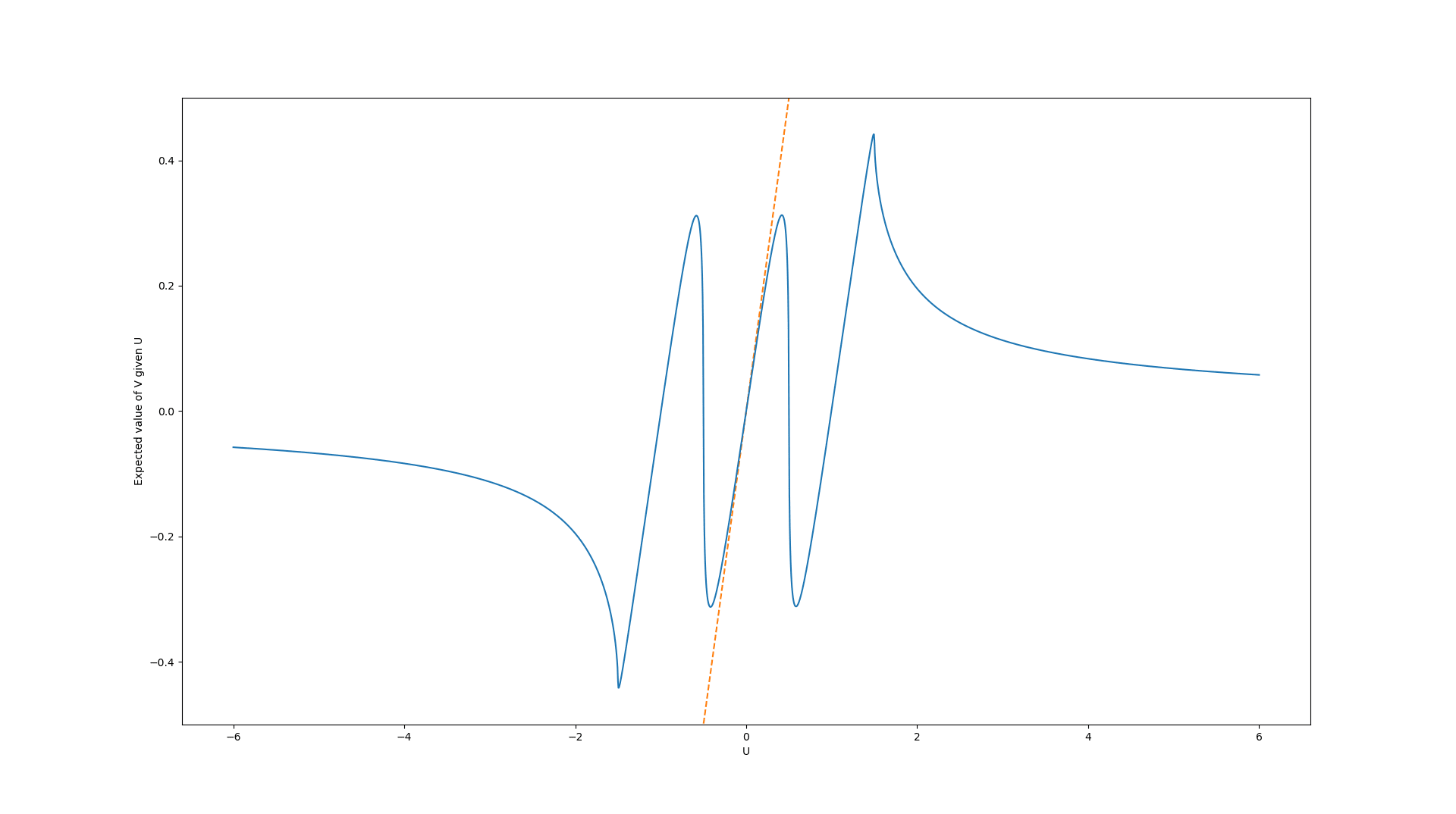
This illustrates that if there are different sources of errors, each with different mean, regressional Goodhart can occur not only in the extreme values, but also in intermediate values in the domain of the proxy function.

What if the agent can’t access the ideal belief distribution?

As discussed, we think that action selection by EU maximization with ideal belief, $a_{\text{Bayes}}^{\star }=\arg {max}_{a^{\prime }\in A}{E}_{\varphi (V|Obs=obs)}V\left(a^{\prime }\right)$, is the best thing to do if feasible, but is infeasible in realistic situations, due to the unavailability of $\varphi$. This raises the question what action selection procedure (algorithm) to employ instead. We search for algorithms with performance (as potentially evaluated by the true value functions for a set of representative situations) as close to the optimal performance reached by EU maximization with ideal belief as possible. In other words: We search for good approximations of action selection by EU maximization with ideal belief.

The naive algorithm and a second-level Goodhart’s law

A salient candidate for the approximation of action selection by EU maximization with ideal belief $\varphi$ is what we call the naive algorithm or naive EU maximization: Action selection by EU maximization with an approximate/​estimated belief $\tilde{\varphi }$:

$a_{\widetilde{\text{Bayes}}}^{\star }=\arg {max}_{a^{\prime }\in A}{E}_{\tilde{\varphi }(V|Obs=obs)}V\left(a^{\prime }\right)$

Curiously, and as observed in Does Bayes Beat Goodhart?, this brings us back into a familiar situation: We found that, in order to optimize $V$ when just knowing $\varphi$, the correct objective to maximize is $E_{\varphi \left(V|\text{Obs}\right)}V$. However, we noticed that the agent can’t typically access this objective and proposed it might maximize $E_{\tilde{\varphi }\left(V|\text{Obs}\right)}V$ instead. Just as in the original situation involving $V$ and $U$, the agent ends up maximizing a proxy of the true objective. This is the recipe for Goodhart’s law. Regardless, we hope that Bayesian reasoning would still reduce the extent of Goodhart’s law in the sense that a solution that avoids it needs to “bridge less of a gap”.

With $Obs=U$, this situation arises in the context of trying to beat Goodhart’s law by Bayesian reasoning, so in some sense on a second level. We could of course attempt to also capture this situation by Bayesian modelling of a meta distribution over $\varphi$ and $\tilde{\varphi }$, but that would just give us a third level Goodhart’s law. Generally, for any meta level of Bayesian reasoning, there is Goodhart’s law one level above. While we hope the Bayesian reasoning on the first level alleviates Goodhart’s law to some degree, our intuition is that further levels of Bayesian reasoning are not helpful. An attempt at an argument for this intuition is that $\varphi$ already captures all the agent’s prior knowledge and $\tilde{\varphi }$ already approximates $\varphi$ to the agent’s best ability. So, if, by replacing $\tilde{\varphi }$ with an expected value of $\varphi$ over the (approximate, not ideal) meta distribution, the agent captures it’s knowledge better, then it must have done a poor job with computing $\tilde{\varphi }$.

In the next section, we will describe a toy example that we will use to test the robustness of the naive approach to Goodhart’s law.

A simulated toy example with difference between ideal and estimated belief distribution

In this example we will analyze how an agent can utilize the true belief distribution $\varphi \left(V|U\right)$ to choose actions to avoid Goodhart’s law, and whether we need this.

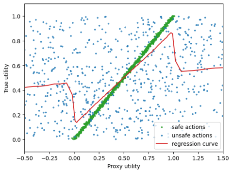
If we knew the true belief distribution $\varphi \left(V|U\right)$ we could label actions as safe or unsafe depending on how correlated V and U are according to $\varphi$. In the figure below we show the extreme example where the true value of “safe actions” are distributed with low variance around the true value mean, while unsafe actions are distributed with high-variance around the true value mean. This is illustrated in the figure below.

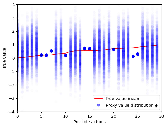
The red curve is a “regression curve” which represents the expected conditional true utility for each proxy utility. This expectation is calculated locally across bins of the proxy utility for visualization purposes.

We can observe that unsafe actions can have two unintended consequences. First, obviously the proxy utilities of unsafe actions are useless as they do not correlate significantly with true utilities. However, the second consequence is that unsafe actions can introduce extremal Goodhart, as the expected true utility (regression curve) decreases for extremal values of the proxy utility.

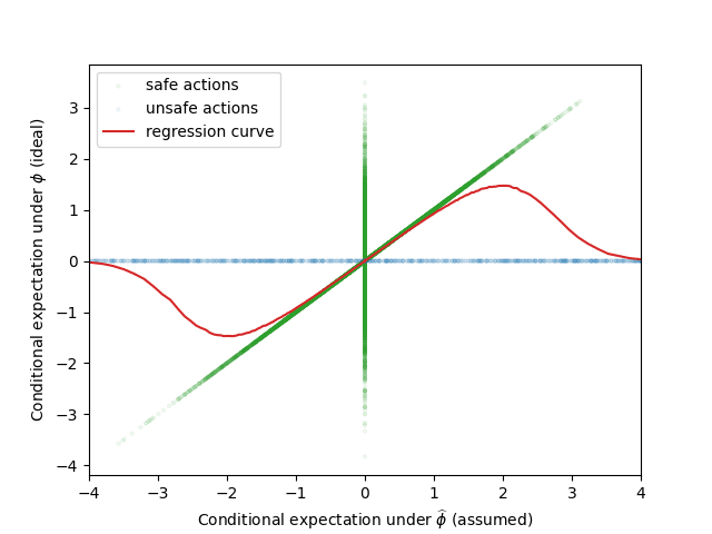
By knowing $\varphi \left(V|U\right)$, we can avoid taking actions for which proxy utilities do not correlate with true utility. Since we do not have knowledge about $\varphi \left(V|U\right)$, we must rely on an estimated belief distribution $\tilde{\varphi }\left(V|U\right)$.

If we assume $\tilde{\varphi }\left(V|U\right)$ is distributed in the same way as $\varphi \left(V|U\right)$, we can observe that, while $\tilde{\varphi }$ and $\varphi$ correlate for safe actions, there is still a Goodhart effect due to the unsafe actions. This example illustrate that approximating $\varphi \left(V|U\right)$ by a prior belief $\tilde{\varphi }\left(V|U\right)$ can still introduce Goodhart. This observations made us consider the usage of soft-optimizers to deal with imperfect information about the prior beliefs.

Conclusion

We investigated concrete examples to build intuitions about Goodhart’s law and found a Bayesian perspective to be helpful for that. We concluded that Goodhart’s law can indeed be beaten by Bayesian reasoning, but that belief misspecification can reintroduce Goodhart’s law. As future work, we are still working on empirical evaluations of soft optimization as an alternative to naive Bayesian expected utility maximization.

Other Results

Stochastic gradient descent as a soft optimizer

Although soft optimizers seem somewhat artificial at first, in fact, a very common soft optimizer is the simplest of optimizers, the standard stochastic gradient descent with a constant time step. The reason for that is exactly because stochastic gradient descent is stochastic, so we can think of it as a sequence of random variables, such that it converges to a stationary distribution around the minimum.

To make this more clear, consider a loss function $l\left(\theta \right)=E\left[L\right(\theta \left)\right]$, with $L\left(\theta \right)$ being a random loss function whose distribution depends on the data. Then, assume we are doing SGD with a step size $\beta$, starting from some ${\theta }_0\sim \pi \left({\theta }_0\right)$. Letting $L_1\left(\theta \right),\dots ,L_B\left(\theta \right)$ be i.i.d. minibatch samples of $L\left(\theta \right)$, then the SGD update forms a Markov chain defined as

${\theta }_{t+1}={\theta }_t-\frac{\beta }{B}{\sum }_{b=1}^B\nabla L_b\left({\theta }_t\right)$

The following is a standard result, which we briefly recap here. We can analyze better this chain by considering

• The CLT approximation $\frac{1}{B}{\sum }_{b=1}^B\nabla L_b\left({\theta }_t\right)\approx \nabla l\left(\theta \right)+B^{-1/2}\Sigma (\theta {)}^{1/2}Z$, where $\Sigma \left(\theta \right)$ be the covariance matrix of $L\left(\theta \right)$, and $Z\sim \mathrm{Normal}(0,I)$.

• That $\beta$ is small enough so that we can consider the stochastic differential limit $d{\theta }_t=-\beta \nabla l\left({\theta }_t\right)+\beta B^{-1/2}\Sigma (\theta {)}^{1/2}d{W}_t$, with $W_t$ denoting the Wiener process.

• That, around the minimum (and under a suitable change of variables) the quadratic approximation $l\left(\theta \right)\approx \frac{1}{2}{\theta }^{T}H\theta$, with $H$ being the Hessian at the minimum, is valid.

• Finally, around the minimum, $\Sigma \left(\theta \right)=\Sigma$ is a constant.

Then our SDE limit becomes $d{\theta }_t=-\beta H{\theta }_{t}dt+\beta B^{-1/2}{\Sigma }^{1/2}d{W}_t$, which we recognize as an OU process, whose stationary distribution is distributed according to $p\left(\theta \right)\propto \exp (-{\theta }^T{A}^{-1}\theta )$, where $A$ is the solution of the equation $AH+HA={\beta }^{-1}{B}^{-1}\Sigma$. We can solve this equation for $A$ by letting $H=Q\mathrm{diag}\left(\lambda \right)Q^T$ be the eigendecomposition of $H$, defining ${\Sigma }_Q:=Q^T\Sigma Q$, and letting^[7]

$A=\frac{\beta }{B}Q\Gamma Q^T,{\Gamma }_{i,j}:=\frac{{\Sigma }_{i,j}^{\left(Q\right)}}{{\lambda }_i+{\lambda }_j}.$

We then conclude that SGD with a constant time step is a soft optimizer that, at convergence, approximately follows a Gaussian distribution whose covariance is proportional to the step size $\beta$ and to the innate covariance $\Sigma$ of $L$, and inversely proportional to $B$ and the eigenvalues of $H$.

An interesting phenomenon arising in high-dimensional probability is that, under usual conditions, the distribution gets highly concentrated in a shell around the mode, called the typical set. In the case of the distribution $p\left(\theta \right)$, we can find this typical set by noticing that, if $\Theta \sim p\left(\theta \right)$, then $\Theta =A^{1/2}Z,Z\sim N(0,I)$, so we find that $Y:=||{\Theta }^T{A}^{-1}\Theta |{|}^2\sim \chi \left(d\right)$, with $\chi \left(d\right)$ being the chi-squared distribution with $d$ degrees of freedom, and $d$ the dimension of the parameter space. Therefore, we find that $E\left[Y\right]=d$ and, using Markov inequality, $P(|Y-k|>td)<2d^{-1}{t}^{-2}$, so the typical set becomes the ellipsoid ${\theta }^T{\Gamma }^{-1}\theta =\beta d/B$, and the relative distance to that set is inversely proportional to $d$.^[8] This implies that, in very high dimensions, not only is constant step SGD soft optimizing the minima, but it in fact rarely gets very near the minima, and just hovers around the typical set.

Of course, SGD with a constant time step is rarely used in real situations, and instead, we use adaptations such as Adam with a schedule for varying the time step. Although the analysis in these cases is somewhat harder, we can conjecture that the general idea still holds, and we still have the same proportionality results. If true, this shows that, when thinking about soft optimizers, we should always remember that soft optimizers are “out there”, already being used all the time.

High probability soft optimizer alternative formulation and proof

Another soft optimizer, that explicitly tries to be a soft optimizer (unlike constant step SGD) is the quantilizer, as proposed by Jessica Taylor. Here, we give an alternative formulation for the quantilizer, one that we believe is more intuitive and slightly more general. To maintain continuity with the previous section, we use a minimization framing, consistent with the SGD discussion, and contrasting to the maximization framing used in the original paper.

Let $l:\Theta \to R$ be a function^[9] to be soft minimized on the state space $\Theta$. We can, for any $t\in R$, consider the sublevel-set $A_{t,l}\subseteq \Theta$ given by $A_{t,l}:=\{\theta \in \Theta ;l(\theta )\le t\}$. Now, assume a prior probability measure $\mu$ on $\Theta$. With it, we can define a function $g_{\mu ,l}:R\to [0,1]$ given by $g_{\mu ,l}\left(t\right)=\mu \left(A_{t,l}\right)$. This function has the following properties:

• For $t\le s$, $A_{t,l}\le A_{t,s}$, therefore $g_{\mu ,l}$ is non-decreasing.

• ${lim}_{t\to -\infty }{g}_{\mu ,l}\left(t\right)=\mu \left(\varnothing \right)=0$, and ${lim}_{t\to -\infty }{g}_{\mu ,l}\left(t\right)=\mu \left(\varnothing \right)=0$.

Therefore, we can define a function $h_{\mu ,l}:[0,1]\to R$, working as a “generalized inverse” of $g_{\pi ,l}$ ($h_{\pi ,l}=g_{\pi ,l}^{-1}$ if $g_{\pi ,l}$ is invertible), by defining $h_{\mu ,l}\left(q\right)=sup\{t\in R;g_{\mu ,f}(t)\le q\}$. With it, we can define the $q$-quantilizer set ${\Theta }_q$ by letting $t_l=h_{\mu ,l}\left(q\right)$ and ${\Theta }_q:=A_{t_q,l}$. Of course, this defines a quantilizer function ${\sigma }_{\mu ,l}:[0,1]\to 2^{\Theta }$ defined as ${\sigma }_{\mu ,l}\left(q\right)={\Theta }_q$. Moreover, we can define the quantilizer distribution function ${\rho }_{\mu ,l}:[0,1]\to P\left(\Theta \right)$ by restricting $\mu$ to ${\Theta }_q$, such that ${\rho }_{\mu ,l}\left(q\right)=\mu (\Theta \cap {\sigma }_{\mu ,l}(q\left)\right)/\mu \left(\Theta \right)=:{\mu }_{q,l}$.

How is this a reformulation? In the original work, the desiderata used is “choosing an action from the set $\{a\in A,E[U\left(W\right(a\left)\right)]\ge t\}$”. In our language (under suitable change to a minimization framing), this is exactly one of the subset levels, and the reordering of the action set and choosing a random variable from $[1-q,1]$ is exactly sampling one of the $q$-best actions based on the prior $\mu$, that is, sampling one of ${\mu }_{q,l}$. We find this explicit reordering of the action space is both awkward, lacking geometric intuition, and hard to generalize to continuous spaces. Instead, we argue that the above reformulation is more intuitive while having the same properties as the original formulation.

We can gain some geometric intuition on quantilizers in $R^d$, by assuming again, that around the minima, we have $l\left(\theta \right)\approx {\theta }^{T}H\theta .$ Then, our quantilizer sets become (approximately) the ellipsoids $A_{t,l}\approx \{{\theta }^{T}H\theta \le t\}$. For large $d$, we again have concentration phenomena in quantilizers. In fact, letting $V\left(A_{t,l}\right)$ be the $d$-dimensional volume of $A_{t,l}$, we find that, for some $\delta <t$, that $V\left(A_{t-\delta ,l}\right)/V\left(A_t\right)=(1-\delta /t{)}^{d/2}$. So, if $\mu$ is approximately uniform around the minima, then for large $d$, and small $q$, almost all of the measure of ${\mu }_{q,l}$ is concentrated around the set $\{\theta H{\theta }^T=t_q\}$. In this case, we conclude that the quantilizer becomes an almost exact quantilizer sampling from the exact $q$-best values of $l\left(\theta \right)$. Of course, unlike in the case of SGD, is not clear that the action set $A$ in the original framing should be modeled as a subset of $R^d$ with all its geometric structure, so whether this result is relevant depends on what is being modeled.

1. ^

   By “ideal” we mean that the agent has arrived at the distribution by Bayesian updates from a well-specified prior, and it includes all the explicit and implicit knowledge available to the agent. From the subjective perspective of the agent, the variables appear (according to some notion that is not very clear to us) to be sampled from this distribution. In the simplest case, the world literally samples from this distribution, e.g. by rolling a die, and the agent has knowledge about the probabilities involved in that sampling process. We are still philosophically confused about what exactly characterizes this ideal distribution and whether there is really only one such distribution in any situation.

2. ^

   With respect to the true value function, which is the value function the designer intends for the agent.

3. ^

   “One possible bayes-beats-goodhart argument is: “Once we quantify our uncertainty with a probability distribution over possible utility functions, the best we can possibly do is to choose whatever maximizes expected value. Anything else is decision-theoretically sub-optimal.” Do you think that the true utility function is really sampled from the given distribution, in some objective sense? And the probability distribution also quantifies all the things which can count as evidence? If so, fine. Alternatively, do you think the probability distribution really codifies your precise subjective uncertainty? Ok, sure, that would also justify the argument.”

4. ^

   Note that we regard $\varphi$ and $\tilde{\varphi }$ as denoting probability measures, joint, conditional and marginal distributions, probability density functions or probability mass functions as convenient.

5. ^

   To show this, we first show $E_{\varphi (U|V=v)}U\left(A^{\star }\right)\ge E_{\varphi (U|V=v)}v\left(A^{\star }\right)$ and then take the expectation over $\varphi \left(V\right)$. Define $\hat{a}:=\arg {max}_{a\in A}v\left(a\right)$. With that, we have $E_{\varphi (U|V=v)}U\left(A^{\star }\right)\ge E_{\varphi (U|V=v)}U\left(\hat{a}\right)=E_{\varphi (U|V=v)}v\left(\hat{a}\right)\ge E_{\varphi (U|V=v)}v\left(A^{\star }\right)$.

   The strict version of this inequality clearly holds if $\varphi \left(U\right(A^{\star })-U(\hat{a}\left)\right)<1$ or $\varphi \left(v\right(A^{\star })=v(\hat{a}\left)\right)<1$.

6. ^

   The exponential distribution has pdf (for $x\ge 0$):

   $f\left(x\right)=\lambda e^{-\lambda x}$

   When values drawn from this distribution are transformed by $g\left(x\right)=x^6$, the pdf of the transformed variable $\sigma$ is given by:

   $\begin{array}{cc}P(\sigma =y)& =f\left(g^{-1}\right(y\left)\right)\frac{d}{dy}{g}^{-1}\left(y\right)\\ & =\frac{\lambda }{6}\exp (-\lambda y^{\frac{1}{6}})y^{-\frac{5}{6}}\text{.}\end{array}$

   Our noise function is Laplace-distributed with location parameter $\mu =0$ and scale parameter $b=0.9\sigma$ and therefore has the pdf (given $\sigma$)

   $P(ϵ=x|\sigma )=\frac{1}{2b}\exp (-\frac{|x-\mu |}{b})=\frac{1}{2\cdot 0.9\sigma }\exp (-\frac{|x|}{0.9\sigma })\text{.}$

   Therefore, if we integrate out $\sigma$, we have

   $\begin{array}{cc}P(ϵ=x)& ={\int }_0^{\infty }d\sigma P(ϵ=x|\sigma )P(\sigma =y)\\ & ={\int }_0^{\infty }d\sigma \frac{1}{2\cdot 0.9\sigma }\exp (-\frac{|x|}{0.9\sigma })\frac{\lambda }{6}\exp (-\lambda {\sigma }^{\frac{1}{6}}){\sigma }^{-\frac{5}{6}}\\ & =\frac{\lambda }{10.8}{\int }_0^{\infty }d\sigma \exp (-\frac{|x|}{0.9\sigma }-\lambda {\sigma }^{\frac{1}{6}}){\sigma }^{-\frac{11}{6}}\\ & =\frac{\lambda }{9}{\int }_0^{\infty }dr\exp (-\frac{|x|}{0.9}{r}^{\frac{6}{5}}-\lambda r^{-\frac{1}{5}})\text{by substituting}r\left(\sigma \right)={\sigma }^{-\frac{5}{6}}\text{,}\end{array}$

   where the last substitution is useful to simplify numerical integration.

7. ^

   This can be shown that the general equation $PX+XP=Y$, for $P$ positive-definite, can be solved using the eigendecomposition $P=Q\Lambda Q^T$, $\Lambda =\mathrm{diag}\lambda$ and letting

   $PX+XP=Y⟹Q^T(PX+XP)Q=Q^{T}YQ$

   $⟹Q^{T}PQ{Q}^{T}XQ+Q^{T}XQ{Q}^{T}PQ=Q^{T}YQ$

   $⟹\Lambda X^{\prime }+X^{\prime }\Lambda =Y^{\prime },X^{\prime }:=Q^{T}XQ,Y^{\prime }:=Q^{T}YQ$

   $⟹{\lambda }_i{X}_{i,j}^{\prime }+{\lambda }_j{X}_{i,j}^{\prime }=Y_{i,j}^{\prime }⟹X_{i,j}^{\prime }=Y_{i,j}^{\prime }({\lambda }_i+{\lambda }_j{)}^{-1}$

8. ^

   Much sharper exponential bounds can be derived, see here.

9. ^

   We assume everything to be well-behaved enough (measurable functions and measurable sets) so we don’t need to do measure theory here.

[beren]

I like this post very much and in general I think research like this is on the correct lines towards solving potential problems with Goodheart’s law—in general Bayesian reasoning and getting some representation of the agent’s uncertainty (including uncertainty over our values!) seems very important and naturally ameliorates a lot of potential problems. The correctness and realizability of the prior are very general problems with Bayesianism but often do not thwart its usefulness in practice although they allow people to come up with various convoluted counterexamples of failure. The key is to have sufficiently conservative priors such that you can (ideally) prove bounds about the maximum degree of goodhearting that can occur under realistic circumstances and then translate these into algorithms which are computationally efficient enough to be usable in practice. People have already done a fair bit of work on this in RL in terms of ‘cautious’ RL which tries to take into account uncertainty in the world model to avoid accidentally falling into traps in the environment.

[Mateusz Bagiński]

People have already done a fair bit of work on this in RL in terms of ‘cautious’ RL which tries to take into account uncertainty in the world model to avoid accidentally falling into traps in the environment.

I would appreciate some pointers to resources