Formalizing Newcombian Problems with Fuzzy Infra-Bayesianism

[Brittany Gelb]

Introduction

In this post, we introduce contributions and supracontributions^[1], which are basic objects from infra-Bayesianism that go beyond the crisp case (the case of credal sets). We then define supra-POMDPs, a generalization of partially observable Markov decision processes (POMDPs). This generalization has state transition dynamics that are described by supracontributions.

We use supra-POMDPs to formalize various Newcombian problems in the context of learning theory where an agent repeatedly encounters the problem. The one-shot version of these problems are well-known to highlight flaws with classical decision theories.^[2] In particular, we discuss the opaque, transparent, and epsilon-noisy versions of Newcomb’s problem, XOR blackmail, and counterfactual mugging.

We conclude by stating a theorem that describes when optimality for the supra-POMDP relates to optimality for the Newcombian problem. This theorem is significant because it gives a sufficient condition under which infra-Bayesian decision theory (IBDT) can approximate the optimal decision. Furthermore, we demonstrate through the examples that IBDT is optimal for problems for which evidential and causal decision theory fail.

Fuzzy infra-Bayesianism

Contributions, a generalization of probability distributions, are defined as follows.

Definition: Contribution

A contribution on a finite set $X$ is a function^[3] $\theta :X\to [0,1]$ such that ${\sum }_{x\in X}\theta \left(x\right)\le 1.$ The set of contributions on $X$ is denoted by ${\Delta }^{C}X$.

Given $A\subseteq X,$ we write $\theta \left(A\right)$ to denote ${\sum }_{x\in A}\theta \left(x\right).$ A partial order on ${\Delta }^{C}X$ is given by ${\theta }_1{\le }_C{\theta }_2$ if for all subsets $A\subseteq X,$ ${\theta }_1\left(A\right)\le {\theta }_2\left(A\right).$ For example, the constant-zero function 0 is a contribution that lies below every element in ${\Delta }^{C}X$ in the partial order. A set of contributions $\Theta$ is downward closed if for all $\theta \in \Theta ,$ ${\theta }^{\prime }{\le }_C\theta$ implies ${\theta }^{\prime }\in \Theta .$ Given $\Theta \subseteq {\Delta }^{C}X,$ the downward closure of $\Theta$ in ${\Delta }^{C}X$ is defined by

$${\Theta }^{\downarrow }:=\{{\theta }^{\prime }\in {\Delta }^{C}X|\exists \theta \in \Theta ,{\theta }^{\prime }{\le }_C\theta \}.$$

Figure 1 illustrates a set of contributions together with its downward closure.

Figure 1: (Purple) Graphical representation of a set $\Theta$ of contributions $\theta$ on $X=\{x_1,x_2\}.$ (Gray shaded region) Elements in the downward closure of $\Theta$ that are not in $\Theta .$

The set of contributions shown in Figure 1 together with its downward closure is an example of a supracontribution, defined as follows.

Definition: Supracontribution

A supracontribution on $X$ is a set of contributions $\Theta \subseteq {\Delta }^{C}X$ such that

1. $0\in \Theta$,

2. $\Theta$ is closed,

3. $\Theta$ is convex, and

4. $\Theta$ is downward closed.

The set of supracontributions on $X$ is denoted by ${\square }^{C}X$.

Figure 2 shows another example of a supracontribution.

Figure 2: Graphical representation of a supracontribution on $X=\{x_1,x_2\}.$

Supracontributions can be regarded as fuzzy sets of distributions, namely sets of distributions in which membership is described by a value in $[0,1]$ rather than $\{0,1\}.$ In particular, the membership $\Gamma (\theta ,\Theta )$ of $\theta \in \Delta X$ in $\Theta \in {\square }^{C}X$ is given by

$$\Gamma (\theta ,\Theta ):=max\{p|p\theta \in \Theta ,p\in [0,1\left]\right\}$$

where $p\theta$ denotes the scaling of $\theta$ by $p.$ See Figure 3 for two examples. Note that $\Gamma$ is well-defined since all supracontributions contain 0. By this viewpoint, supracontributions can be seen as a natural generalization of credal sets, which are “crisp” or ordinary sets of distributions.

Figure 3: (Left) A distribution $\theta$ and a supracontribution $\Theta$ that is the downward closure of a different distribution. Here $\Gamma (\theta ,\Theta )=0.$ (Right) A distribution $\theta$ and a supracontribution $\Theta$ with $\Gamma (\theta ,\Theta )=p>0.$

There is a natural embedding $\tau :\square X\to {\square }^{C}X$ of credal sets on $X$ into the space of supracontributions on $X.$ Let ${\perp }_X:=\left\{0\right\}.$ Define $\tau \left(\Theta \right):={\Theta }^{\downarrow }\cup {\perp }_X.$ Note that under this definition, $\tau \left(\varnothing \right)={\perp }_X$ (and otherwise the union with ${\perp }_X$ in the definition of $\tau$ is redundant).

Figure 4: (Purple line segment) A credal set $\Theta$ on $X=\{x_1,x_2\}$, and (gray shaded region) the supracontribution $\tau \left(\Theta \right)={\Theta }^{\downarrow }.$

Generalizing the notion of expected value, we write $E_{\theta }\left[L\right]:={\sum }_{x\in X}\theta \left(x\right)L\left(x\right).$ We define expectation (similarly as in the crisp case) as the max over all expectations for elements of the supracontribution. By definition, a supracontribution is closed and thus this notion of expectation is well-defined.

Definition: Expectation with respect to a supracontribution

Given a continuous function $L:X\to [0,1]$ and $\Theta \in {\square }^{C}X,$ define the expectation of $L$ with respect to $\Theta$ by

$$E_{\Theta }\left[L\right]:=\underset{\theta \in \Theta }{max}{E}_{\theta }\left[L\right].$$

Let $\tilde{\Theta }\subseteq {\Delta }^{C}X$ denote a non-empty set of contributions. Then ${sup}_{\theta \in \tilde{\Theta }}{E}_{\theta }\left[L\right]={max}_{\theta \in \overline{\text{ch}(\tilde{\Theta }{)}^{\downarrow }}}{E}_{\theta }\left[L\right]$ where $\text{ch}$ denotes convex hull and $\overline{\cdot }$ denotes closure. Therefore, in the context of optimization we may always replace a non-empty set of contributions by the supracontribution obtained by taking the convex, downward, and topological closure.

Recall that environments in the classical theory and in crisp infra-Bayesianism have type $(A\times O{)}^{\ast }\times A\to \Delta O.$ We generalize this notion to the fuzzy setting using semi-environments.^[4]

Definition: Semi-environment

A semi-environment is a map of the form $\mu :(A\times O{)}^{\ast }\times A\to {\Delta }^{C}O.$

The interaction of a semi-environment and a policy $\pi :(A\times O{)}^{\ast }\rightharpoonup A$ determines a contribution on destinies ${\mu }^{\pi }\in {\Delta }^C(A\times O{)}^{\omega }.$^[5]

Definition: (Fuzzy) law

A (fuzzy) law generated by a set of semi-environments $E$ is a map $\Lambda :\Pi \to {\square }^C(A\times O{)}^{\omega }$ such that for all $\pi \in \Pi ,$ $\Lambda \left(\pi \right)={\overline{\text{ch}\left(\right\{{\mu }^{\pi }|\mu \in E\left\}\right)}}^{\downarrow }$ where $\text{ch}$ denotes convex hull and $\overline{\cdot }$ denotes closure.

Fuzzy Supra-POMDPs

Our tool for formalizing Newcombian problems using the mathematical objects described in the last section is fuzzy supra-POMDPs, a generalization of partially observable Markov decision processes (POMDPs). Given a set of states $S$ and a contribution $\theta \in {\Delta }^C\left(S\right),$ the missing probability mass, $1-\theta \left(S\right),$ can be interpreted as the probability of a logical contradiction.

Under a fuzzy supra-POMDP model, uncertainty of the initial state is described by an initial supracontribution over states. Similarly to the state transition dynamics of a crisp supra-POMDP as defined in the preceding post, the state transition dynamics of a fuzzy supra-POMDP are multivalued. Given a state and action, the transition suprakernel returns a supracontribution, and the true dynamics are described by any element of the supracontribution.

A significant feature of fuzzy supra-POMDPs is that for some state $s$ and action $a,$ we may have $T(s,a)={\perp }_S,$ which corresponds to a logical contradiction in which the state transition dynamics come to a halt. We use this feature to model Newcombian problems where it is assumed there is a perfect predictor Omega predicting an agent’s policy. When an action deviates from the predicted policy (which is encoded in the state), the transition kernel returns ${\perp }_S.$

We formally define fuzzy supra-POMDPs as follows.

Definition: Fuzzy supra-POMDP

A fuzzy supra-partially observable Markov decision process (supra-POMDP) is a tuple $(S,{\Theta }_0,A,O,T,B)$ where

• $S$ is a set of states,

• ${\Theta }_0\in {\square }^{C}S$ is an initial supracontribution over states,

• $A$ is a set of actions,

• $O$ is a set of observations,

• $T:S\times A\to {\square }^{C}S$ is a transition suprakernel,^[6]

• $B:S\to O$ is an observation mapping.

Defining laws from fuzzy supra-POMDPs

Every fuzzy supra-POMDP defines a (fuzzy) law. The construction is similar to the construction of a crisp law given a crisp supra-POMDP, which is discussed in the preceding post. A copolicy to a fuzzy supra-POMDP is a map $\sigma :(S\times A{)}^{\ast }\to {\Delta }^{C}S$ that is consistent with the transition suprakernel. More specifically, given a history of states and actions, the transition kernel determines a supracontribution from the most recent state and action. The copolicy can be thought of as a map that selects a contribution from that supracontribution.

Definition: Copolicy to a fuzzy supra-POMDP

Let $M=(S,{\Theta }_0,A,O,T,B)$ be a fuzzy supra-POMDP. A map $\sigma :(S\times A{)}^{\ast }\to {\Delta }^{C}S$ is an $M$-copolicy if

1. $\sigma \left(ϵ\right)\in {\Theta }_0$ for the empty string $ϵ,$ and

2. For all non-empty strings $hsa\in (S\times A{)}^{\ast }$, $\sigma \left(hsa\right)\in T(s,a)$.

An $M$-copolicy $\sigma :(S\times A{)}^{\ast }\to {\Delta }^{C}S$ and the observation map $B:S\to O$ of $M$ together determine a semi-environment ${\mu }_{\sigma }:(A\times O{)}^{\ast }\times A\to {\Delta }^{C}O.$ Let

$$E_M:=\left\{{\mu }_{\sigma }|\sigma \text{is an}M\text{-copolicy}\right\}.$$

Then $M$ defines the law generated by $E_M.$

Formalizing Newcombian problems

In this section, we give a mathematical definition for Newcombian problems and describe how to model Newcombian problems using fuzzy supra-POMDPs.

Let $O$ denote a set of observations. Given a time-horizon $H\in N,$ let $O^{<H}$ denotes strings in $O$ of length less than $H.$ Let ${\Pi }_H$ denote the set of horizon-$H$ policies, i.e. maps of the form $\pi :O^{<H}\to A.$

Definition: Newcombian problem with horizon $H$

A Newcombian problem with horizon $H\in N$ is a map $\nu :{\Pi }_H\times O^{<H}\to \Delta O$ together with a loss function $L:(A\times O{)}^H\to [0,1].$

Intuitively speaking, given a policy and a sequence of observations, a Newcombian problem specifies some distribution that describes uncertainty about the next observation. This framework allows for a mathematical description of an environment in which there is a perfect predictor Omega and a distribution over observations that depends on the policy that Omega predicts.

Optimal policy for a Newcombian problem

Similar to how the interaction of a policy and an environment produce a distribution over destinies, a Newcombian problem $\nu$ and a policy $\pi \in {\Pi }_H$ together determine a distribution on outcomes, ${\nu }^{\pi }\in \Delta (A\times O{)}^H.$ The policy that minimizes expected loss with respect to this distribution is said to be a $\nu$-optimal policy.

Definition: Optimal policy for a Newcombian problem

A policy $\pi \in {\Pi }_H$ is optimal for a Newcombian problem if $\pi \in {\text{argmin}}_{\pi \in {\Pi }_H}{E}_{{\nu }^{\pi }}\left[L\right]$.

If $\pi \in {\Pi }_H$ is optimal for $\nu ,$ then $E_{{\nu }^{\pi }}\left[L\right]$ is said to be the optimal loss for $\nu .$

Formalism for multiple episodes

In order to discuss learning, we consider the case of multiple episodes where an agent repeatedly encounters the Newcombian problem.

Given some number of episodes $n>1,$ let $\Pi :O^{<nH}\to A$ denote the set of multi-episode policies. A multi-episode policy $\pi \in \Pi$ gives rise to a sequence of single-episode policies $\left\{{\pi }_k|{\pi }_k\right(o_0\dots o_m):=\pi (o_0\dots o_{kH+m}),m\le H-1{\}}_{k=0}^{n-1}\subseteq {\Pi }_H.$

By means of this sequence of single-episode policies, a Newcombian problem $\nu$ and a multi-episode policy together determine a distribution on outcomes over multiple episodes, which we also denote by ${\nu }^{\pi }\in \Delta (A\times O{)}^{nH}.$

The loss function $L:(A\times O{)}^H\to [0,1]$ can be naturally extended to multiple episodes by considering the mean loss per episode. In particular, if $n\in N$ and $h\in (A\times O{)}^{nH}$ is given by $h=a_0{o}_0\dots a_{nH-1}{o}_{nH-1},$ then the mean loss over $n$ episodes is defined as

$$L_n\left(h\right):=\frac{1}{n}\sum _{k=0}^{n-1}L(a_{kH}{o}_{kH}\cdots a_{kH+H-1}{o}_{kH+H-1}).$$

It is also possible to extend the loss to multiple episodes by considering the sum of the per-episode loss with a geometric time discount. In this case, the total loss is defined by

$$L_n^{\gamma }\left(h\right)=(1-\gamma )\sum _{k=0}^{n-1}{\gamma }^{k}L(a_{kH}{o}_{kH}\cdots a_{kH+H-1}{o}_{kH+H-1}).$$

The fuzzy supra-POMDP associated with a Newcombian problem

In this section, we describe how to model iterated Newcombian problems (i.e. repeated episodes of the problem) by a fuzzy supra-POMDP. We work in the iterated setting since this allows us to talk about learning. Examples are given in the following section.

The state space, initialization, and observation mapping

Let $\nu :{\Pi }_H\times O^{<H}\to \Delta O$ (together with $L:(A\times O{)}^H\to [0,1]$) be a Newcombian problem. Let $S={\Pi }_H\times O^{<H}.$ Informally speaking, the state always encodes both a policy and a sequence of observations.

Let the initial supracontribution over states be ${\Theta }_0={\top }_{{\Pi }_H\times \lambda }:=\overline{\text{ch}\left(\right\{{\delta }_{\pi \times \left\{\lambda \right\}}|\pi \in {\Pi }_H\}}{)}^{\downarrow }$ where $\lambda$ denotes the empty observation. This supracontribution represents complete ambiguity over the policy (and certainty over the empty observation).

The observation mapping $B:S\to O$ simply returns the most recent observation datum from a state, i.e.$B(\pi ,o_0\dots o_n)=o_n$ for non-empty observation strings. If the observation string of the state is the empty string $\lambda ,$ then $B(\pi ,\lambda )$ may be chosen arbitrarily.

The transition suprakernel

We start with an informal description of the transition suprakernel $T:S\times A\to {\square }^{C}S,$ which is defined in three cases. In short:

1. If the action is compatible with the policy encoded by the state, then $T$ is determined by $\nu .$

2. If the action is not compatible with the policy encoded by the state, then $T$ returns ${\perp }_S.$

3. If the end of the episode is reached, then $T$ returns ${\top }_{{\Pi }_H\times \lambda }.$

To elaborate, we have the following three cases.

1. The action is compatible with the policy encoded by the state, and the time-step is less than the horizon, i.e. the episode is not yet complete. In this case, the policy datum of the state remains the same with certainty, whereas $\nu$ determines a distribution over next observations. This distribution determines a distribution over next states. The transition suprakernel returns the downward closure of this distribution. (Here the downward closure is used simply to obtain a supracontribution.)

2. The action is not compatible with the policy encoded by the state, and the time-step is less than the horizon. This case is a logical contradiction, and thus $T$ returns ${\perp }_S.$

3. The time-step is equal to the horizon, i.e. the end of the episode has been reached. The transition suprakernel returns the initial supracontribution ${\top }_{{\Pi }_H\times \lambda }$ again, which represents complete ambiguity over the policy for the next episode (and certainty over the empty observation).

We now formally define $T:S\times A\to {\square }^{C}S.$ Given $(\pi ,o_0\dots o_n)\in S$ such that $n<H-1,$ define $\text{pref}(\pi ,o_0\dots o_n):O\to S$ by $\text{pref}(\pi ,o_0\dots o_n)\left(q\right):=(\pi ,o_0\dots o_{n}q)$. Namely, $\text{pref}(\pi ,o_0\dots o_n)$ appends a given observation to the prefix of observations $o_0\dots o_n$ and returns the corresponding state. Let ${\text{pref}}_{\ast }$ denote the pushforward of $\text{pref}.$

Define

$$T(\pi ,o_0\dots o_n,a):=\{\begin{array}{cc}\left\{\text{pref}\right(\pi ,o_0\dots o_n{)}_{\ast }\left(\nu \right(\pi ,o_0\dots o_n\left)\right){\}}^{\downarrow }& \text{if}a=\pi (o_0\dots o_n)\text{and}n<H-1,\\ {\perp }_S& \text{if}a\ne \pi (o_0\dots o_n)\text{and}n<H-1,\\ {\top }_{{\Pi }_H\times \lambda }& \text{if}n=H-1.\end{array}$$

Examples of Newcombian problems

In this section, we explain how to formalize various Newcombian problems using the fuzzy supra-POMDP framework. We provide the most detail for the first two examples

Newcomb’s Problem

We first consider Newcomb’s Problem. In this problem, there are two boxes: Box A, a transparent box that always contains $1K, and Box B, an opaque box that either contains $0 or $1M. An agent can choose to “one-box”, meaning that they only take Box B, or “two-box”, meaning they take both boxes. A perfect predictor Omega fills Box B with $1M if and only if Omega predicts that the agent will one-box.

Evidential decision theory (EDT) prescribes that an agent should choose the action that maximizes the expected utility conditioned on choosing that action. Thus, EDT recommends one-boxing because choosing to one-box can be seen as evidence that Box B contains $1M. This is the case even though the correlation is spurious, i.e. choosing to one-box does not cause there to be $1M in Box B. We will see that IBDT also recommends one-boxing. In comparison to EDT, causal decision theory (CDT)^[7] prescribes that an agent should only take into account what an action causes to happen and therefore recommends two-boxing.

Let $O=\{\lambda ,o_{\$1K},o_{\$1M},o_{\$1.001M}\}$ where $\lambda$ denotes the empty observation and the remaining observations represent the total amount of money received.

Let $A=\{a_1,a_2\},$ where $a_1$ corresponds to one-boxing and $a_2$ corresponds to two-boxing. Without loss of generality, ${\Pi }_H=\{{\pi }_1,{\pi }_2\}$ where ${\pi }_1\left(\lambda \right)=a_1$ and ${\pi }_2\left(\lambda \right)=a_2.$

Then $\nu :{\Pi }_H\times O^{<H}\to \Delta O$ is defined by

$$\nu ({\pi }_1,\lambda )={\delta }_{o_{\$1M}},\text{and}$$$$\nu ({\pi }_2,\lambda )={\delta }_{o_{\$1K}}.$$

The loss of an episode $L:(A\times O)\to [0,1]$ is defined by

$$L\left(ao\right)=\{\begin{array}{c}0\text{if}o=o_{\$1M}\\ 1\text{if}o=o_{\$1K}.\end{array}$$

(We don’t define $L\left(ao\right)$ for $o=o_{\$1.001M}$ because under this model, this observation never occurs.)

Note that $E_{{\nu }^{{\pi }_1}}\left[L\right]=1\cdot 0=0,$ and $E_{{\nu }^{{\pi }_2}}\left[L\right]=1\cdot 1=1.$ Therefore, ${\pi }_1$ is $\nu -$optimal.

We now consider the corresponding supra-POMDP $M_{\nu }.$ The transition suprakernel is given by

$$T\left(\right({\pi }_1,\lambda ),a_1)=\{{\delta }_{({\pi }_1,o_{\$1M})}{\}}^{\downarrow },$$$$T\left(\right({\pi }_1,\lambda ),a_2)={\perp }_S,$$$$T\left(\right({\pi }_2,\lambda ),a_2)=\{{\delta }_{({\pi }_2,o_{\$1K})}{\}}^{\downarrow },$$$$T\left(\right({\pi }_2,\lambda ),a_1)={\perp }_S,\text{and}$$$$T\left(\right({\pi }_1,o_{\$1.001M}),\cdot )=T\left(\right({\pi }_2,o_{\$1K}),\cdot )=\text{ch}({\delta }_{({\pi }_1,\lambda )},{\delta }_{({\pi }_2,\lambda )}{)}^{\downarrow }={\top }_{{\Pi }_H\times \lambda }.$$

Figure 5 shows the state transition graph of $M_{\nu }.$ Notably, it is not possible under $M_{\nu }$ for an agent to two-box when Box B is full (the left branch in Figure 5). This is assured by the fact that $T\left(\right({\pi }_1,\lambda ),a_2)={\perp }_S.$

Figure 5: State transitions of the supra-POMDP that represents Newcomb’s problem.

The interaction of $M_{\nu }$ and ${\pi }_1$ produces a supracontribution over outcomes given by ${\Theta }_1=\{{\delta }_{a_1{o}_{\$1M}}{\}}^{\downarrow }.$ Similarly, the interaction of $M_{\nu }$ and ${\pi }_2$ produces the supracontribution ${\Theta }_2=\{{\delta }_{a_2{o}_{\$1K}}{\}}^{\downarrow }.$

Then the expected loss for ${\pi }_1$ in one round is

$$\begin{array}{cc}{E}_{M_{\nu }^{{\pi }_1}}\left[L\right]& :=E_{{\Theta }_1}\left[L\right]\\ & =\underset{\theta \in {\Theta }_1}{max}{E}_{\theta }\left[L\right]\\ & =E_{{\delta }_{a_1{o}_{\$1M}}}\left[L\right]\\ & =0.\end{array}$$

Similarly, the expected loss for ${\pi }_2$ in one round is

$$\begin{array}{cc}{E}_{M_{\nu }^{{\pi }_2}}\left[L\right]& :=E_{{\Theta }_2}\left[L\right]\\ & =\underset{\theta \in {\Theta }_2}{max}{E}_{\theta }\left[L\right]\\ & =E_{{\delta }_{a_2{o}_{\$1K}}}\left[L\right]\\ & =1.\end{array}$$

From another viewpoint, the optimal (worst-case from the agent’s perspective) copolicy ${\sigma }_{{\pi }_i}$ to ${\pi }_i$ initializes the state to $({\pi }_i,\lambda )$ for $i=1,2,$ i.e.${\sigma }_{{\pi }_i}\left(\lambda \right)={\delta }_{({\pi }_i,\lambda )}.$ In other words, the policy encoded in the state chosen by the copolicy matches the policy of the agent. The law defined by this supra-POMDP is equivalent to an ordinary environment in which one-boxing results in observing a full box and two-boxing results in observing an empty box.

We see from the above calculations that the optimal policy for $M_{\nu }$ is ${\pi }_1,$ and moreover ${\pi }_1$ achieves the $\nu$-optimal loss. This analysis holds for any number of episodes. This is significant because if a learning agent has $M^{\nu }$ in their hypothesis space, then they must converge to one-boxing if they are to achieve low regret for the iterated Newcomb’s problem.

Note that for this example, we have only used what might be considered the most basic supracontributions, namely $\top ,$ $\perp ,$ and the downward closure of a single probability distribution. In the next example, we will see the full power of supracontributions.

XOR Blackmail

In this section we describe how to use a supra-POMDP to model the XOR blackmail problem. For a more in depth discussion of XOR blackmail, see e.g. Toward Idealized Decision Theory §2.1 (Soares and Fallenstein, 2015) and Cheating Death in Damascus §2 (Levinstein and Soares, 2020).

The problem is given as follows. Suppose there is a 1% probability that an agent’s house may have a termite infestation that would cause $1M in damages. A blackmailer can predict the agent and also knows whether or not there is an infestation. The blackmailer sends a letter stating that exactly one of the following is true, if and only if the letter is truthful:

1. There are no termites, and you will pay $1K, or

2. There are termites, and you will not pay.

The agent can then accept or reject the blackmail. Note that as stated, the probability of blackmail depends on the agent’s policy. Because policies are encoded in the state space of the associated supra-POMDP, we are able to model this. EDT recommends accepting the blackmail because accepting blackmail is evidence that there is not an infestation, even though this correlation is spurious (i.e. accepting the blackmail does not causally influence whether or not there is an infestation). On the other hand, CDT recommends rejecting the blackmail. Thus we see that these two decision theories are split across the two examples that we have seen so far and neither always recommends an optimal action. We now see that IBDT does recommend the optimal action again.

Let $O=\{\lambda ,o_B,o_{NB},o_{\$0},o_{-\$\text{1K}},o_{-\$\text{1M}}\},$ where $\lambda$ denotes the empty observation, $o_B$ represents receiving the blackmail, $o_{NB}$ represents not receiving the blackmail, and the remaining observations represent the various monetary outcomes.

Let $A=\{a_a,a_r\},$ where $a_a$ corresponds to accepting the blackmail and $a_r$ corresponds to rejecting the blackmail. Without loss of generality, ${\Pi }_H=\{{\pi }_a,{\pi }_r\}$ where ${\pi }_a:(\dots o_B)=a_a$ and ${\pi }_r(\dots o_B)=a_r.$

Interpreting the statement of the problem, we define $\nu :{\Pi }_H\times O^{<H}\to \Delta O$ as follows:

$$\nu ({\pi }_a,\lambda )\left(o_B\right)=0.99\text{and}\nu ({\pi }_a,\lambda )\left(o_{NB}\right)=0.01,$$$$\nu ({\pi }_a,o_B)\left(o_{-\$1K}\right)=1,$$$$\nu ({\pi }_a,o_{NB})\left(o_{-\$1M}\right)=1,$$$$\nu ({\pi }_r,\lambda )\left(o_{NB}\right)=0.99\text{and}\nu ({\pi }_r,\lambda )\left(o_B\right)=0.01,$$$$\nu ({\pi }_r,o_{NB})\left(o_{\$0}\right)=1,\text{and}$$$$\nu ({\pi }_r,o_B)\left(o_{-\$1M}\right)=1.$$

We normalize in order to define the loss of an episode $L:(A\times O{)}^H\to [0,1]$ by

$$L(a_0{o}_0\dots a_{H-1}{o}_{H-1})=\{\begin{array}{cc}0& \text{if}{o}_{H-1}=o_{\$0}\\ 0.001& \text{if}{o}_{H-1}=o_{-\$1K}\\ 1& \text{if}{o}_{H-1}=o_{-\$1M}.\end{array}$$

Note that $E_{{\nu }^{{\pi }_a}}\left[L\right]=0.99\cdot 0.001+0.01\cdot 1,$ whereas $E_{{\nu }^{{\pi }_r}}\left[L\right]=0.99\cdot 0+0.01\cdot 1.$ Therefore ${\pi }_r$ is $\nu -$optimal.

We now consider the corresponding supra-POMDP $M_{\nu }.$ The state transitions of $M_{\nu }$ are summarized in Figure 6. We first define the transition suprakernel on ${\Pi }_H\times \lambda .$ Using $\nu ,$ we have

$$T({\pi }_a,\lambda )=\{0.99{\delta }_{({\pi }_a,o_B)}+0.01{\delta }_{({\pi }_a,o_{NB})}{\}}^{\downarrow }\text{and}$$$$T({\pi }_r,\lambda )=\{0.99{\delta }_{({\pi }_r,o_{NB})}+0.01{\delta }_{({\pi }_r,o_B)}{\}}^{\downarrow }.$$

We now consider the next level of the supra-POMDP. Since ${\pi }_a\left(o_B\right)=a_a,$

$$T\left(\right({\pi }_a,o_B),a_a)=\{{\delta }_{({\pi }_a,o_B{o}_{-\$1K})}{\}}^{\downarrow }\text{and}$$$$T\left(\right({\pi }_a,o_B),a_r)={\perp }_S.$$

Here we see that when the action is $a_a$, which is consistent with the policy of the state ${\pi }_a$, the transition kernel returns the downward closure of a distribution specified by $\nu .$ On the other hand, when the action is $a_r$, which is not consistent with ${\pi }_a$, the transition kernel returns ${\perp }_S$.

The action does not matter when there is no blackmail (i.e. both actions are consistent with the policy), so

$$T\left(\right({\pi }_a,o_{NB}),a_a)=T\left(\right({\pi }_a,o_{NB}),a_r)=\{{\delta }_{({\pi }_a,o_{NB}{o}_{-\$1M})}{\}}^{\downarrow }.$$

A similar analysis for ${\pi }_r$ yields

$$T\left(\right({\pi }_r,o_{NB}),a_a)=T\left(\right({\pi }_r,o_{NB}),a_r)=\{{\delta }_{({\pi }_r,o_{NB}{o}_{\$0})}{\}}^{\downarrow },$$$$T\left(\right({\pi }_r,o_B),a_a)={\perp }_S,\text{and}$$$$T\left(\right({\pi }_r,o_B),a_r)=\{{\delta }_{({\pi }_r,o_B{o}_{-\$1M})}{\}}^{\downarrow }.$$

Then on the final level: for all $s\in \left\{{\pi }_a\right\}\times \{o_B{o}_{-\$1K},o_{NB}{o}_{-\$1M}\}\cup \left\{{\pi }_r\right\}\times \{o_{NB}{o}_{\$0},o_B{o}_{-\$1M}\},$ define

$$T(s,\cdot )=\text{ch}({\delta }_{({\pi }_a,\lambda )},{\delta }_{({\pi }_r,\lambda )}{)}^{\downarrow }={\top }_{{\Pi }_H\times \lambda }.$$

Figure 6: State transitions of the supra-POMDP that represents XOR Blackmail.

We now consider the expected loss of each policy for $M_{\nu }.$ The interaction of $M_{\nu }$ and ${\pi }_a$ produces a supracontribution over outcomes given by $\Theta =\text{ch}\{{\theta }_0,{\theta }_1{\}}^{\downarrow }$ where

$${\theta }_0=0.99\left({\delta }_{o_B{a}_a{o}_{-\$1K}}\right)+0.01\left({\delta }_{o_{NB}{a}_a{o}_{-\$1M}}\right),\text{and}$$$${\theta }_1=0.99\left({\delta }_{o_{NB}{a}_a{o}_{\$0}}\right).$$

Here, ${\theta }_0$ arises from the interaction of ${\pi }_a$ with the branch starting with state $({\pi }_a,\lambda ).$ We have a probability distribution in this case because ${\pi }_a$ is always consistent with itself, which is the policy encoded in the states of this branch. On the other hand, the contribution ${\theta }_1$ arises from the interaction of ${\pi }_a$ with the branch starting with state $({\pi }_r,\lambda ).$ In the case of blackmail, ${\pi }_a$ and ${\pi }_r$ disagree on the action and thus a probability mass of 0.01 is lost on this branch.

Therefore, the expected loss for ${\pi }_a$ in one round is given by

$$\begin{array}{cc}{E}_{M_{\nu }^{{\pi }_a}}\left[L\right]& :=E_{\Theta }\left[L\right]\\ & =\underset{\theta \in \Theta }{max}{E}_{\theta }\left[L\right]\\ & =max\left\{E_{{\theta }_0}\right[L],E_{{\theta }_1}[L\left]\right\}\\ & =max\{0.99\cdot 0.001+0.01\cdot 1,0.99\cdot 0\}\\ & =0.99\cdot 0.001+\mathrm{0.01.}\end{array}$$

Another way to view this calculation is that the optimal $M_{\nu }$-copolicy $\sigma$ initializes the state to $({\pi }_a,\lambda ),$ meaning $\sigma \left(\lambda \right)={\delta }_{({\pi }_a,\lambda )}.$

By a similar calculation,

$$E_{M_{\nu }{}^{{\pi }_r}}\left[L\right]=max\{0.01\cdot 1,0.99\cdot 0+0.01\cdot 1\}=\mathrm{0.01.}$$

Therefore, the optimal policy for $M_{\nu }$ is also ${\pi }_r$, i.e. under this formulation it is optimal to reject the blackmail. This analysis holds for any number of episodes. Moreover, the optimal loss for $M_{\nu }$ is equal to the optimal loss for $\nu .$ This is significant because if a learning agent has $M_{\nu }$ in their hypothesis space, then they must converge to rejecting the blackmail if they are to achieve low regret for the iterated Newcombian problem.

Counterfactual Mugging

We now consider the problem of counterfactual mugging. In this problem, a perfect predictor (the “mugger”) flips a coin. If the outcome is heads, the mugger asks the agent for $100, at which point they can decide to pay or not pay. Otherwise, they give the agent $10K if and only if they predict the agent would have paid the $100 if the outcome was heads.

Both CDT and EDT recommend not paying, and yet we will see that IBDT recommends to pay the mugger.

Let $O=\{\lambda ,o_H,o_T,o_{\$10K},o_{-\$100},o_{\$0}\},$ where $o_H$ represents heads, $o_T$ represents tails, and the remaining (non-empty) observations represent the various monetary outcomes. Let $A=\{a_p,a_{np}\},$ where $a_p$ represents paying the mugger and $a_{np}$ represents not paying the mugger. Without loss of generality, ${\Pi }_H=\{{\pi }_p,{\pi }_{np}\}$ where ${\pi }_p(\dots o_H)=a_p$ and ${\pi }_{np}(\dots o_H)=a_{np}.$

Let $\alpha :=1-\frac{100}{10,100}$. We normalize^[8] to define the loss $L:(A\times O{)}^H\to [0,1]$ of an episode by

$$L(a_0{o}_0\dots a_{H-1}{o}_{H-1})=\{\begin{array}{cc}0& \text{if}{o}_{H-1}=o_{\$10K}\\ \alpha & \text{if}{o}_{H-1}=o_{\$0}\\ 1& \text{if}{o}_{H-1}=o_{-\$100}.\end{array}$$

Note that $E_{{\nu }^{{\pi }_p}}\left[L\right]=0.5\left(1\right)+0.5\left(0\right)=0.5,$ whereas $E_{{\nu }^{{\pi }_{np}}}\left[L\right]=0.5\left(\alpha \right)+0.5\left(\alpha \right)=\alpha .$ Therefore, ${\pi }_p$ is $\nu$-optimal.

The state transitions of $M_{\nu }$ are shown in Figure 7.

Figure 7: State transitions of the supra-POMDP that represents counterfactual mugging.

We have

$$E_{M_{\nu }^{{\pi }_p}}\left[L\right]=max\{0.5\cdot 1+0.5\cdot 0,0.5\cdot \alpha \}=0.5,$$

whereas

$$E_{M_{\nu }^{{\pi }_{np}}}\left[L\right]=max\{0.5\cdot 0,0.5\cdot \alpha +0.5\cdot \alpha \}=\alpha .$$

Therefore, the optimal policy for $M^{\nu }$ is also ${\pi }_p$, i.e. under this formulation it is optimal to pay the mugger.

Transparent Newcomb’s Problem

We now consider Transparent Newcomb’s Problem. In this problem, both boxes of the original problem are transparent. We consider three versions. See Figure 11 in the next section for a summary of the decision theory recommendations.

Empty-box dependent

In the empty-box dependent version, a perfect predictor Omega leaves Box B empty if and only if Omega predicts that the agent will two-box upon seeing that Box B is empty.

Let $O=\{\lambda ,o_E,o_F,o_{\$1M},o_{\$1K},o_{\$1.001M}\}.$ Here $o_E$ corresponds to observing an empty box and $o_F$ corresponds to observing a full box. Let $A=\{a_1,a_2\},$ where $a_1$ corresponds to one-boxing and $a_2$ corresponds to two-boxing.

Without loss of generality, ${\Pi }_H=\{{\pi }_{1,1},{\pi }_{1,2},{\pi }_{2,1},{\pi }_{2,2}\}$ where ${\pi }_{i,j}(\dots o_E)=a_i$ and ${\pi }_{i,j}(\dots o_F)=a_j$ for $i,j\in \{1,2\}.$ Namely, the policies are distinguished by the action chosen upon observing an empty or full box.

Let $\alpha :=1-\frac{1,000,000}{1,001,000}$. Define $L:(A\times O{)}^H\to [0,1]$ by

$$L(a_0{o}_0\dots a_{H-1}{o}_{H-1})=\{\begin{array}{cc}0& \text{if}{o}_{H-1}=o_{\$1.001M}\\ \alpha & \text{if}{o}_{H-1}=o_{\$1M}\\ 1& \text{if}{o}_{H-1}=o_{\$1K}.\end{array}$$

The state transition graph of the supra-POMDP $M_{\nu }$ representing this problem is shown in Figure 8.

Figure 8: State transitions of the supra-POMDP $M_{\nu }$ that represents the empty-box dependent transparent Newcomb’s problem.

We now consider the expected loss in one round for each policy interacting with $M_{\nu }.$ Similarly to the original version of Newcomb’s problem, the optimal copolicy to a policy ${\pi }_{i,j}$ initializes the state to $({\pi }_{i,j},\lambda )$, meaning the policy encoded in the state chosen by the copolicy matches the true policy of the agent.

We have

$$\begin{array}{cc}{E}_{M_{\nu }^{{\pi }_{1,1}}}\left[L\right]& =max\left\{L\right(\dots o_{\$1M}),E_0[L],E_0[L],E_0[L\left]\right\}\\ & =max\{\alpha ,0,0,0\}\\ & =\alpha ,\\ E_{M_{\nu }^{{\pi }_{1,2}}}\left[L\right]& =max\left\{E_0\right[L],L(\dots o_{\$1.001M}),E_0[L],E_0[L\left]\right\}\\ & =max\{0,0,0,0\}\\ & =0,\\ E_{M_{\nu }^{{\pi }_{2,1}}}\left[L\right]& =max\left\{L\right(\dots o_{\$1M}),E_0[L],L(\dots o_{\$1K}),L(\dots o_{\$1K}\left)\right\}\\ & =max\{\alpha ,0,1,1\}\\ & =1,\text{and}\\ E_{M_{\nu }^{{\pi }_{2,2}}}\left[L\right]& =max\left\{E_0\right[L],L(\dots o_{\$1.001M}),L(\dots o_{\$1K}),L(\dots o_{\$1K}\left)\right\}\\ & =max\{0,0,1,1\}\\ & =1.\end{array}.$$

Therefore, the optimal policy for $M_{\nu }$ is ${\pi }_{1,2},$ meaning it is optimal to one-box upon observing an empty box and to two-box upon seeing a full box. Note that ${\pi }_{1,2}$ is also the $\nu$-optimal policy.

Full-box dependent

In the full-box dependent version, Omega (a perfect predictor) puts $1M in Box B if and only if Omega predicts that the agent will one-box upon seeing that Box B is full. This example does not satisfy pseudocausality (discussed below), and therefore we will see that there is an inconsistency between the optimal policies for the supra-POMDP $M_{\nu }$ and the Newcombian problem $\nu .$

Let $O=\{\lambda ,o_E,o_F,o_{\$1M},o_{\$1K},o_{\$0}\},$ and $A=\{a_1,a_2\}.$ Without loss of generality, we again have ${\Pi }_H=\{{\pi }_{1,1},{\pi }_{1,2},{\pi }_{2,1},{\pi }_{2,2}\}$ where ${\pi }_{i,j}(\dots o_E)=a_i$ and ${\pi }_{i,j}(\dots o_F)=a_j$ for $i,j\in \{1,2\}.$

The state transition graph of the supra-POMDP $M_{\nu }$ representing this problem is shown in Figure 9.

Figure 9: State transitions of the supra-POMDP that represents the full-box dependent transparent Newcomb’s problem.

Define $L:(A\times O{)}^H\to [0,1]$ by

$$L(a_0{o}_0\dots a_{H-1}{o}_{H-1})=\{\begin{array}{cc}0& \text{if}{o}_{H-1}=o_{\$1M}\\ 0.999& \text{if}{o}_{H-1}=o_{\$1K}\\ 1& \text{if}{o}_{H-1}=o_{\$0}.\end{array}$$

Then

$$\begin{array}{cc}{E}_{M_{\nu }^{{\pi }_{1,1}}}\left[L\right]& =max\{0,0,1,0\}\\ & =1,\text{and}\\ E_{M_{\nu }^{{\pi }_{1,2}}}\left[L\right]& =max\{0,0,1,0\}\\ & =1.\end{array}$$

Furthermore,

$$\begin{array}{cc}{E}_{M_{\nu }^{{\pi }_{2,1}}}\left[L\right]& =max\{0,0,0,0.999\}\\ & =0.999,\text{and}\\ E_{M_{\nu }^{{\pi }_{2,2}}}\left[L\right]& =max\{0,0,0,0.999\}\\ & =\mathrm{0.999.}\end{array}$$

Therefore, the optimal policies for the supra-POMDP $M_{\nu }$ are ${\pi }_{2,2}$ and ${\pi }_{2,1}.$ From another perspective, the optimal copolicy to ${\pi }_{1,j}$ for $j=1,2$ initializes the state to $({\pi }_{1,2},\lambda )$. The optimal copolicy to ${\pi }_{2,j}$ for $j=1,2$ initializes the state to $({\pi }_{2,2},\lambda )$. As a result, an agent can achieve low regret on $M_{\nu }$ and either one- or two-box upon observing the full box. In particular, for all policies they will learn to expect an empty box.

On the other hand, the optimal policies for the Newcombian problem $\nu$ are ${\pi }_{1,1}$ and ${\pi }_{2,1}$. To see this, note that $\text{supp}\left({\nu }^{{\pi }_{1,1}}\right)=\text{supp}\left({\nu }^{{\pi }_{2,1}}\right)=\left\{o_F{a}_1{o}_{\$1M}\right\},$ $\text{supp}\left({\nu }^{{\pi }_{1,2}}\right)=\left\{o_E{a}_1{o}_{\$0}\right\},$ and $\text{supp}\left({\nu }^{{\pi }_{2,2}}\right)=\left\{o_E{a}_2{o}_{\$1K}\right\}.$ Then $E_{{\nu }^{{\pi }_{1,1}}}\left[L\right]=E_{{\nu }^{{\pi }_{2,1}}}\left[L\right]=0,$ whereas $E_{{\nu }^{{\pi }_{1,2}}}\left[L\right]=1$ and $E_{{\nu }^{{\pi }_{2,2}}}=\mathrm{0.999.}$ The inconsistency between the optimal policies for $M_{\nu }$ and $\nu$ is a result of the fact that this Newcombian problem fails to satisfy pseudocausality, a condition we describe in the last section.

Epsilon-noisy full-box dependent

We now consider a variant of the full-box dependent version in which we assume that Omega is not a perfect predictor. In this case, Omega also puts $1M in Box B with probability $ϵ\in (0,0.999)$ when the agent will two-box upon seeing that Box B is full.

Figure 10 shows the state transitions starting from states $({\pi }_{1,2},\lambda )$ and $({\pi }_{2,2},\lambda ).$ (The full state transition graph is the graph in which the the two right-most paths of the graph of Figure 9 are replaced by the trees in Figure 10.)

Figure 10: Modified branches of the two right-most paths in the state transitions in Figure 6 for the epsilon-noisy variant of the full-box dependent Newcomb’s problem.

Let $\alpha :=1-\frac{1,000,000}{1,001,000}$ and $\beta :=1-\frac{1,000}{1,001,000}.$ Define $L:(A\times O{)}^H\to [0,1]$ by

$$L(a_0{o}_0\dots a_{H-1}{o}_{H-1})=\{\begin{array}{cc}0& \text{if}{o}_{H-1}=o_{\$1.001M}\\ \alpha & \text{if}{o}_{H-1}=o_{\$1M}\\ \beta & \text{if}{o}_{H-1}=o_{\$1K}\\ 1& \text{if}{o}_{H-1}=o_{\$0}.\end{array}$$

A distinguishing feature of the supra-POMDP for this problem (compared to the other problems we have considered) is that the optimal policy for $M_{\nu }$ depends on the number of episodes. In the case of one episode, the optimal copolicy to ${\pi }_{2,1}$ and ${\pi }_{2,2}$ is the same. Namely, $\sigma \left(\lambda \right)={\delta }_{({\pi }_{2,2},\lambda )}.$ Then the expected loss for one episode is

$$E_{M_{\nu }^{{\pi }_{2,1}}}\left[L\right]=E_{M_{\nu }^{{\pi }_{2,2}}}\left[L\right]=(1-ϵ)\beta .$$

We consider the extension of $L$ given by the mean per-episode loss. For two episodes, the optimal copolicy to ${\pi }_{2,1}$ and ${\pi }_{2,2}$ again has $\sigma \left(\lambda \right)={\delta }_{({\pi }_{2,2},\lambda )}.$ The interaction of $\sigma$ and ${\pi }_{2,1}$ produces a supracontribution over $(A\times O{)}^{2H}$ given by ${\Theta }_{2,1}=\text{ch}\{\theta {\}}^{\downarrow }$ where $h=\lambda o_E{a}_2{o}_{\$1K}\lambda o_E{a}_2{o}_{\$1K}$^[9] and $\theta =(1-ϵ{)}^2{\delta }_h.$ Then the expected mean loss for ${\pi }_{2,1}$ over two episodes is

$$E_{M_{\nu }^{{\pi }_{2,1}}}\left[L_2\right]=E_{{\Theta }_{2,1}}\left[L_2\right]=\beta (1-ϵ{)}^2.$$

On the other hand, the interaction of $\sigma$ and ${\pi }_{2,2}$ produces a supracontribution over $(A\times O{)}^{2H}$ given by ${\Theta }_{2,2}=\text{ch}\{{\theta }^{\prime }{\}}^{\downarrow }$ where ${\theta }^{\prime }\in \Delta (O\times A{)}^2$ is defined by

$$\begin{array}{cc}{\theta }^{\prime }\left(\lambda o_E{a}_2{o}_{\$1K}\lambda o_E{a}_2{o}_{\$1K}\right)& =(1-ϵ{)}^2\\ {\theta }^{\prime }\left(\lambda o_E{a}_2{o}_{\$1K}\lambda o_F{a}_2{o}_{\$1.001M}\right)& =ϵ(1-ϵ)\\ {\theta }^{\prime }\left(\lambda o_F{a}_2{o}_{\$1.001M}\lambda o_E{a}_2{o}_{\$1K}\right)& =ϵ(1-ϵ)\\ {\theta }^{\prime }\left(\lambda o_F{a}_2{o}_{\$1.001M}\lambda o_F{a}_2{o}_{\$1.001M}\right)& ={ϵ}^2.\end{array}$$

Then

$$\begin{array}{cc}{E}_{M_{\nu }^{{\pi }_{2,2}}}\left[L_2\right]& =E_{{\Theta }_{2,2}}\left[L_2\right]\\ & =\frac{1}{2}\left(2\beta \right(1-ϵ{)}^2+2\beta ϵ(1-ϵ))\\ & =\beta (1-ϵ).\end{array}$$

More generally, for any number $n\in N$ of episodes, the worst-case copolicy to ${\pi }_{2,2}$ has $\sigma \left(ϵ\right)={\delta }_{({\pi }_{2,2},\lambda )}.$ As a result, $E_{M_{\nu }^{{\pi }_{2,2}}}\left[L_n\right]=\beta (1-ϵ)$ for all $n\in N.$

On the other hand, over $n$ episodes, the copolicy to ${\pi }_{2,1}$ that always has $\sigma \left(\lambda \right)={\delta }_{({\pi }_{2,2},\lambda )}$ results in an expected mean loss of $\beta (1-ϵ{)}^n,$ which tends to zero as $n\to \infty .$ The copolicy to ${\pi }_{2,1}$ that instead has $\sigma \left(\lambda \right)={\delta }_{({\pi }_{2,1},\lambda )}$ on most episodes results in a mean expected loss that converges to $\alpha .$ Therefore, for sufficiently many episodes, ${\pi }_{2,1}$ is the optimal policy for $M_{\nu },$ and moreover the optimal loss for $M_{\nu }$ converges to the optimal loss for $\nu .$

Summary of decision theory recommendations

In Figure 11, we summarize the extent to which each decision theory makes optimal recommendations on the example problems.

Figure 11: Table indicating for which problems CDT, EDT, and IBDT make optimal recommendations. For readability, a blank entry indicates that the recommendation is not optimal. Note that EDT is ill-posed when it involves conditioning on a probability zero event. The only example where IBDT fails to be optimal or optimal in the limit does not satisfy pseudocausality.

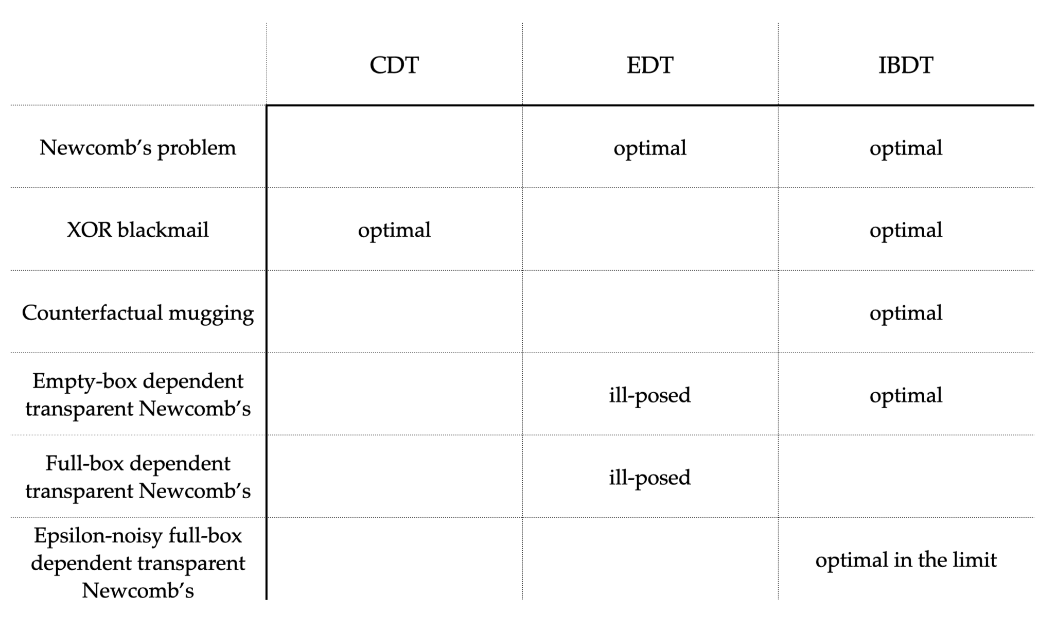
Readers familiar with decision theory will observe that IBDT can be seen as an approximation to functional decision theory, which makes optimal recommendations across all the examples here. IBDT has the advantage of being well-defined in the sense that it can be run as code in an agent learning from the environment.

Pseudocausality

In this section, we define a condition (pseudocausality) that holds for all of the Newcombian problems discussed above, except for the (non-noisy) full-box dependent transparent Newcomb’s problem. We then state a theorem that illuminates the significance of this condition. In particular, pseudocausality allows one to translate optimality from the supra-POMDP $M_{\nu }$ to optimality for the corresponding Newcombian problem $\nu .$ Intuitively, pseudocausality means that there does not exist a suboptimal policy for $\nu$ such that the optimal policy and the suboptimal policy disagree only on events that are probability zero under the suboptimal policy.

To formally define pseudocausality, we consider the set of outcomes $C_{\pi }$ that are compatible with a given policy $\pi .$ Namely, define

$$C_{\pi }:=\{h\in (A\times O{)}^H|\forall \text{prefixes}{h}^{\prime }a\in (A\times O{)}^{\ast }\times A\text{of}h,a=\pi (h^{\prime }\left)\right\}.$$

In other words, $h\in C_{\pi }$ if the sequence of actions in $h$ agrees with $\pi ,$ whereas the observations can be arbitrary.

Definition: Pseudocausality

A Newcombian problem $\nu$ satisfies pseudocausality if there exists a $\nu$-optimal policy ${\pi }_{\ast }\in {\Pi }_H$ such that for all $\pi \in {\Pi }_H$ if $\text{supp}\left({\nu }^{\pi }\right)\subseteq C_{{\pi }_{\ast }},$ then $\pi$ is also optimal for $\nu .$

An example where pseudocausality fails

To see why pseudocausality fails for the full-box dependent transparent Newcomb’s problem, recall that the optimal policies for $\nu$ are ${\pi }_{1,1}$ and ${\pi }_{2,1}.$ We have

$$C_{{\pi }_{1,1}}=o_E{a}_1\times O\cup o_F{a}_1\times O$$

and

$$C_{{\pi }_{2,1}}=o_E{a}_2\times O\cup o_F{a}_1\times O.$$

However,

$$\text{supp}\left({\nu }^{{\pi }_{1,2}}\right)=\left\{o_E{a}_1{o}_{\$0}\right\}\subset C_{{\pi }_{1,1}},$$

and

$$\text{supp}\left({\nu }^{{\pi }_{2,2}}\right)=\left\{o_E{a}_2{o}_{\$1K}\right\}\subset C_{{\pi }_{2,1}},$$

but ${\pi }_{1,2}$ and ${\pi }_{2,2}$ are not optimal for $\nu .$

We leave it to the reader to check that all other examples discussed in this post satisfy pseudocausality.

Theorem on pseudocausality and optimality

The significance of pseudocausality is given by the next theorem. It states that if pseudocausality holds for a Newcombian problem $\nu$, then the optimal loss for the corresponding fuzzy supra-POMDP $M_{\nu }$ converges to the optimal loss for the Newcombian problem. Furthermore, given a time discount $\gamma \in [0,1),$ if a $\gamma -$indexed family of policies is optimal for $M_{\nu }$ in the $\gamma \to 1$ limit, then the family is also optimal for $\nu$ in the $\gamma \to 1$ limit.

Theorem [Alexander Appel (@Diffractor), Vanessa Kosoy (@Vanessa Kosoy)]:

Let $\nu :{\Pi }_H\times O^{<H}\to \Delta O$ be a Newcombian problem that satisfies pseudocausality. Then

$$\underset{\gamma \to 1}{lim}|\underset{\pi \in \Pi }{min}{E}_{M_{\nu }^{\pi }}\left[L^{\gamma }\right]-\underset{\pi \in \Pi }{min}{E}_{{\nu }^{\pi }}\left[L^{\gamma }\right]|=0.$$

Furthermore, if $\{{\pi }_{\gamma }{\}}_{\gamma \in [0,1)}$ is a family of policies such that ${lim}_{\gamma \to 1}{E}_{M_{\nu }^{{\pi }_{\gamma }}}\left[L^{\gamma }\right]-{min}_{\pi \in \Pi }{E}_{M_{\nu }^{\pi }}\left[L^{\gamma }\right]=0,$ then

$$\underset{\gamma \to 1}{lim}{E}_{{\nu }^{{\pi }_{\gamma }}}\left[L^{\gamma }\right]-\underset{\pi \in \Pi }{min}{E}_{{\nu }^{\pi }}\left[L^{\gamma }\right]=0.$$

See the proof section for the proof.

Acknowledgements

Many thanks to Vanessa Kosoy, Marcus Ogren, and Mateusz Bagiński for their valuable feedback on initial drafts. Vanessa’s video lecture on formalizing Newcombian problems was also very helpful in writing this post.

1. ^

   Previously called ultracontributions.

2. ^

   To make comparisons, we briefly review these decision theories, but this is not the focus of the post.

3. ^

   More generally, if $X$ is a measurable space, we define a contribution $\theta$ to be a measure such that $\theta \left(X\right)\le 1.$

4. ^

   This terminology is motivated by the notions of semimeasures and semi-probabilities as discussed in An Introduction to Universal Artificial Intelligence (M. Hutter, D. Quarel, and E. Catt).

5. ^

   Here it is necessary to use the more general definition of a contribution as a measure.

6. ^

   Here suprakernel simply means a map in which the range is the set of supracontributions over some set.

7. ^

   For more detail, see Toward Idealized Decision Theory §2.2 (Soares and Fallenstein, 2015) and Cheating Death in Damascus §3 (Levinstein and Soares, 2020).

8. ^

   If $o_{H-1}=o_{\$q},$ then $L(a_0{o}_0\dots a_{H-1}{o}_{H-1})=1-\frac{q+100}{10,100}.$

9. ^

   As a technicality, we always assume that the empty action is taken at the beginning of an episode.