A Primer on Matrix Calculus, Part 1: Basic review
Consider whether this story applies to you. You went through college and made it past linear algebra and multivariable calculus, and then began your training for deep learning. To your surprise, much of what they taught you in the previous courses is not very useful to the current subject matter.
And this is fine. Mathematics is useful in its own right. You can expect a lot of stuff isn’t going to show up on the deep learning final, but it’s also quite useful for understanding higher mathematics.
However, what isn’t fine is that a lot of important stuff that you do need to know was omitted. In particular, the deep learning course requires you to know matrix calculus, a specialized form of writing multivariable calculus (mostly differential calculus). So now you slog through the notation, getting confused, and only learning as much as you need to know in order to do the backpropagation on the final exam.
This is not how things should work!
Matrix calculus can be beautiful in its own right. I’m here to find the beauty for myself. If I may find it beautiful, then perhaps I will find new joy in reading those machine learning papers. And maybe you will too.
Therefore, I dedicate the next few posts in this sequence to covering this paper, which boldly states that it is, “an attempt to explain all the matrix calculus you need in order to understand the training of deep neural networks.” All the matrix calculus we need? Perhaps it’s enough to understand training neural networks, but it isn’t enough matrix calculus for deep learning more generally — I just Ctrl-F’d and found no instance of “hessian”!
Since it’s clearly not the full picture, I will supplement my posts with material from chapter 4 of the Deep Learning Book, and Wikipedia.
This subsequence of my daily insights sequence will contain three parts. The first part is this post, the introduction. For the posts in the sequence I have outlined the following rubric:
Part 1 (this one) will be reviewing some multivariable calculus and will introduce the matrix calculus notation.
Part 2 will cover Jacobians, derivatives of element-wise binary operators, derivatives involving scalar expansions, vector sum reduction, and some common derivatives encountered in deep learning.
Part 3 will cover the hessian matrix, higher order derivatives and Taylor approximations, and we will step through an example of applying the chain rule in a neural network.
First, what’s important to understand is that most of the calculus used in deep learning is not much more advanced than what is usually taught in a first course in calculus. For instance, there is rarely any need for understanding integrals.
On the other hand, even though the mathematics itself is not complicated, it takes the form of specialized notation, enabling us to write calculus using large vectors and matrices, in contrast to a single variable approach.
Given this, we might as well start from somewhat of a beginning, with limits, and then build up to derivatives. Intuitively, a limit is a way of filling in the gaps of certain functions by finding what value is “approached” when we evaluate a function in a certain direction. The formal definition for a limit given by the epsilon-delta definition, which was provided approximately 150 years after the limit was first introduced.
Let be a real valued function on a subset of the real numbers. Let be a limit point of and let be a real number. We say that if for every there exists a such that, for all , if then . For an intuitive explanation of this definition, see this video from 3Blue1Brown.
It is generally considered that this formal definition is too cumbersome to be applied every time to elementary functions. Therefore, introductory calculus courses generally teach a few rules which allow students to quickly evaluate the limits of functions that we are familiar with.
I will not attempt to list all of the limit rules and tricks, since that would be outside of the scope of this single blog post. That said, this resource provides much more information than what would be typically necessary for succeeding in a machine learning course.
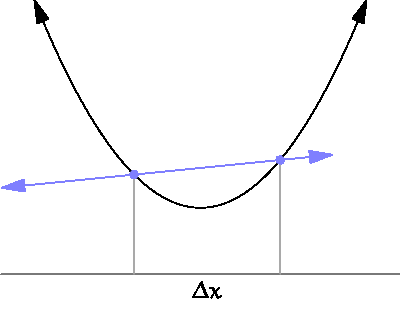
The derivative is defined on real valued functions by the following definition. Let be a real valued function, then the derivative of at is written . The intuitive notion of a derivative is that it measures the slope of a function at a point . Since slope is traditionally defined as the rate of change between two points, it may first appear absurd to a beginner how we can measure slope at a single point. But this absurdity can be visually resolved by viewing the following GIF
Just as in the case of limits, we are usually not interested in applying the formal definition to functions except when pressed. Instead we have a list of common derivative rules which can help us simplify derivatives of common expressions. Here is a resource which lists common differentiation rules.
In machine learning, we are most commonly presented with functions which whose domain is multi-dimensional. That is, instead of taking the derivative of a function where is a real valued variable, we are interested in taking the derivative of functions where is a vector, which is intuitively something that can be written as an ordered list of numbers.
To see why we work with vectors, consider that we usually interested in finding a local minimum of the loss function of a neural network (a measure of how badly the neural network is performing) where the parameters of the neural network are written as an ordered list of numbers. During training, we can write the loss function as a function of its weights and biases. In general, all of deep learning can be reduced notation-wise to simple multidimensional functions, and compositions of those simple functions.
Therefore, in order to understand deep learning, we must understand the multidimensional generalization of the derivative, the gradient. First, in order to construct the gradient, however, we must briefly consider the notion of partial derivatives. A quick aside, I have occasionally observed that some people seem at first confused by partial derivatives, imagining them to some type of fractional notion of calculus.
Do not be alarmed. As long as you understand what a derivative is in one dimension, partial derivatives should be a piece of cake. A partial derivative is simply a derivative of a function with respect to a particular variable, with all the other variables held constant. To visualize, consider the following multidimensional function that I have ripped from Wikimedia.
Here, we are taking the partial derivative of the function with respect to where is held constant at and the axis represents the co-domain of the function (ie. the axis that is being mapped to). I think about partial derivatives in the same way as the image above, by imagining taking a slice of the function in the x-direction, and thereby reducing the function to one dimension, allowing us to take a derivative. Symbolically, we can evaluate a function’s partial derivative like this: say . If we want to take the derivative of with respect to , we can treat the ’s in that expression as constants and write . Here, the symbol is a special symbol indicating that we are taking the partial derivative rather than the total derivative.
The gradient is simply the column vector of partial derivatives of a function. In the previous example, we would have the gradient as . The notation I will use here is that the gradient is written as for some function. The gradient is important because it generalizes the concept of slope to a higher dimension. Whereas the single variable derivative provided us the slope of the function at a single point, the gradient provides us a vector which points in the direction of greatest ascent at a point and whose magnitude is equal to the rate of increase in this direction. Also, just as a derivative allows us to construct a local linear approximation of a function about a point, the gradient allows us to construct a linear approximation of a multivariate function about a point in the form of a hyperplane. From this notion of a gradient, we can “descend” down a loss function by repeatedly subtracting the gradient starting at some point, and in the process find neural networks which are better at doing their assigned tasks.
In deep learning we are often asked to take the gradient of a function (this notation is just saying that we are mapping from a space of matrices to the real number line). This may occur because the function in question has its parameters organized in the form of an by matrix, representing for instance the strength of connections from neuron to neuron . In this case, we treat the gradient exactly as we did before, by collecting all of the partial derivatives. There is no difference, except in notation.
Some calculus students are not well acquainted with the proof for why the gradient points in the direction of greatest ascent. Since it is simply a list of partial derivatives, this fact may seem surprising. Nonetheless, this fact is what makes the gradient centrally important in deep learning, so it is therefore worth repeating here.
In order to see why the gradient points in the direction of steepest ascent, we first need a way of measuring the ascent in a particular direction. It turns out that multivariable calculus offers us such a tool. The directional derivative is the rate of change of a function along a direction . We can imagine the directional derivative as being conceptually similar to the partial derivative, except we would first change the basis while representing the function, and then evaluate the partial derivative with respect to a basis vector which is on the span of . Similar to the definition for the derivative, we define the directional derivative as
Additionally, we can employ the multivariable chain rule to re-write the directional derivative in a way that uses the gradient. In single variable calculus, the chain rule can be written as . In the multivariable case, for a function , we write where is the partial derivative of with respect to its th argument. This can be simplified by employing the following notation, which uses a dot product: .
If we rewrite the definition of the directional derivative as , and then apply the multivariate chain rule to this new formulation, we find that .
Given that , the unit vector which maximizes this dot product is the unit vector which points in the same direction as . This previous fact can be proven by a simple inspection of the definition of the dot product between two vectors, which is that where is the angle between the two vectors. is maximized when . For more intuition on how to derive the dot product, I recommend this video from 3Blue1Brown. I also recommend this one for intuitions on why the gradient points in the direction of maximum increase.
For more depth I recommend this part four of this pdf text. For even more depth I recommend this book (though I have not read it). For even more depth, I recommend seeing the footnote below. For even more depth than that, perhaps just try to complete a four year degree in mathematics.
Even this 1962 page behemoth called a book, intended to introduce all of the mathematics needed for a computer science education, includes very little information on integration, despite devoting full chapters to topics like tensor algebras and topology. However, if or when I blog about probability theory, integration will become relevant again.
If this wasn’t enough for you, alternatively you can view the 3Blue1Brown video on derivatives.
Interestingly, fractional calculus is indeed a real thing, and is very cool.
For a proof which is does not use the multivariable chain rule, see here. I figured given the primacy of the chain rule in deep learning, it is worth mentioning now.
Awesome! I’m with you so far. :)
This was one of the main things I struggled with when trying to get through some of the early examples in the Deep Learning book. “The Matrix Cookbook” was a decent reference manual but was lacking context and explanation. Thanks for writing this!
The provided link does not work. The site appears to have been moved to a new address: https://sites.science.oregonstate.edu/math/home/programs/undergrad/CalculusQuestStudyGuides/SandS/lHopital/index.html
In this paragraph:
>In single variable calculus, the chain rule can be written as ddxf(g(x))=f′(g(x))g′(x). In the multivariable case, for a function f:Rk→R, we write ddxf(g(x))=∑ki=1ddxgi(x)Dif(g(x)) where Di is the partial derivative of f with respect to its ith argument. This can be simplified by employing the following notation, which uses a dot product: ddxf(g(x))=∇f⋅g′(x).
What does gi() stand for?
My understanding that g maps g:Rm→Rk and gi indicates i-th element of a vector that g produces.
Is that the right way to think about it?