Visual Exploration of Gradient Descent (many images)
If you (understandably) think “this post is too long, ain’t nobody got time for that!” I suggest scrolling to ~the middle of the post and at least check out the Mandelbrot Training Animation(s). I think they’re pretty neat.
After going through ~half of the ARENA curriculum, I couldn’t stop myself from taking a few days off and just exploring what happens in a small neural network during gradient descent. I’m summarizing that little adventure in this not-so-little post. Hard to say how far my findings and newly won intuitions generalize beyond this particular case, but at the very least it led to some nice-looking pictures.
What I Did
I trained a small neural network (<100 neuron MLPs) to learn complex number multiplication. Technically, I didn’t train one, but a whole bunch of them. Here are some of the questions I wanted to answer:
How well can models of different sizes learn complex number multiplication?
What does the learned function actually look like?
What does the loss landscape look like when rendered in different ways?
What does the trajectory of the network weights and biases throughout the training process look like?
If we take a bunch of untrained randomly initialized networks, what distribution of losses do we obtain?
How does this distribution change after 1, 10, 100 training epochs?
How much does initialization matter for ultimate performance of a network?
What does the Mandelbrot set look like when rendered with the learned function instead of real complex number multiplication?
As this was rather explorative and not super systematic, much of what I did was rather improvised. For instance, I didn’t do thorough hyperparameter exploration in any sense, but just manually tried out different numbers (for e.g. batch size, training set size and learning rate) and ended up with a configuration that seemed to perform well enough. As the function I’m training on is quite simple and the networks are small, most training runs finished within a few seconds and the entire project fit well within <$10 worth of cloud compute.
Throughout this post, I’ll typically start with a question, giving readers a chance to reflect on their expectations to test their intuition, before summarizing what I found.
Caveat: Pretty much all I did here was vibe-coded using the Google Colab Gemini integration (and occasionally help from Claude whenever Gemini got stuck). So I can’t entirely guarantee the code doesn’t contain any stupid mistakes and perhaps very occasionally doesn’t quite do what I think it does. That being said, most of what I found seems pretty plausible to me and/or I continued investigating up to a point where things clearly worked out the way they should. The exception to this is probably the Loss Landscape section towards the end, which stands on shakier ground. If you want to check the code, or run any of the experiments yourself, please PM me and I’ll gladly share the colab notebook.
What is complex number multiplication?
I can imagine many lesswrong readers are broadly familiar with the concept, but for those who are not, here’s a very basic introduction to complex numbers. Basically, while real numbers move on a 1-dimensional “ray” of numbers, complex numbers can be interpreted as points in a 2D space (the complex plane). So, a complex number x consists of two components (or coordinates), called its real and its imaginary part, which can be written as rex + imx i, where i is a constant with the property that i² = −1. Here, rex can be interpreted as “pointing in the direction of real numbers”, while i (and thereby also imx i) would be orthogonal to that, “pointing in the direction of imaginary numbers”. Defining complex numbers like this, addition of two complex numbers is trivial—you can just add real parts and imaginary parts separately (like vector addition in R²). Multiplication is also pretty straightforward when doing it in closed form algebraically: for two complex numbers x and y, you get
(rex + imx i) × (rey + imy i) = rex rey + rex imy i + imx rey i + imx imy i²
But since i² is defined as −1, we can turn this into:
= rex rey + rex imy i + imx rey i—imx imy
= (rex rey—imx imy) + (rex imy + imx rey)i
And so we end up with a new complex number, where its real part (rex rey—imx imy) and imaginary part (rex imy + imx rey) can be straightforwardly calculated with simple addition and multiplication.
One neat “application” of complex numbers is that they allow computing (and thereby rendering visually) some interesting “fractals” like the Mandelbrot set—which we’ll do later on.
The neural network(s) that I’ve trained are not able to express complex number multiplication fully, as they cannot multiply activations but only add them[1]. Hence, what the networks are going to learn, will always just be an approximation of this function rather than the real math behind it.
Network Architecture
As I wanted to train a network on complex number multiplication, I needed 4 inputs (real and imaginary part of two complex numbers) and 2 outputs (real and imaginary part of the result). I varied the number and width of hidden layers throughout my experiments.
Some other implementation and training details:
Adam optimizer
Most of the time I’d use ReLU as activation function, sometimes SiLU
MSE loss
I used 4k pieces of training data (input output pairs), sampled initially from a normal distribution with a standard deviation of 2 around the origin, with an 80:20 train test split
I mostly used a learning rate of 0.01 and no weight decay
Batch size of 512
All done in Google Colab with pytorch
Trying Out Different Model Sizes
At first, I trained models with a few different hidden layer setups to see how well they perform:
No hidden layers, connecting input to output directly
One hidden layer, [10] neurons, ReLU as activation function
Two hidden layers, [10, 10] neurons
Three hidden layers, [20, 30, 20] neurons
Three hidden layers, [20, 30, 20] neurons, using SiLU instead of ReLU
Feel free to come up with some hypotheses on how these will perform, either relative to each other or even what MSE loss to expect. I trained all of these for 150 epochs each (learning rate of 0.01, 4096 * 0.8 training samples).
Results
Unsurprisingly, larger models performed better than smaller ones. SiLU helped a lot. In all cases, train loss was lower than test loss, but they were reasonably close, to the networks generalized well enough (but then again, with a function as smooth as complex number multiplication, it would be surprising if there was no generalization).
Here are the train and test losses I obtained after 150 epochs for each of the models:
| Model | Hidden Layers | Train Loss | Test Loss |
0 | [] | 6.2571 | 7.6424 |
1 | [10] ReLU | 3.1443 | 3.7585 |
2 | [10, 10] ReLU | 1.6828 | 2.2726 |
3 | [20, 30, 20] ReLU | 0.1662 | 0.3403 |
4 | [20, 30, 20] SiLU | 0.0225 | 0.1108 |
5 | [20, 30, 20] SiLU (1000 epochs) | 0.0036 | 0.0262 |
I won’t show all the details, but here’s the exemplary loss curve of model 3 ([20, 30, 20] hidden layers using ReLU):
Eyeballing it, it appears that this particular model went through ~3 phases during training, with the first ~6 epochs going through a very steep drop, then dropping more slowly but ~linearly until epoch ~30-40, and then just very slowly getting closer towards 0. I didn’t look more deeply into these phases though. This was also not a general pattern for the other models (although the very broad pattern of steep drop at first that abruptly turns flat holds for all of them).
I likely could have trained any of these models for much longer to reduce the loss further. E.g. the last model, after its 1000 epochs, did not plateau yet. I also could have used more training samples (or dynamically generated training data instead of fixed samples) to improve generalization and reduce the gap between train and test loss.
Neuron Count
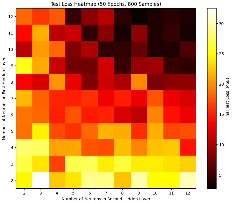
Taking the case of 2 hidden layers, I was wondering how the neuron count in these layers would affect the loss. So I made a grid of [2…12] x [2…12] and trained (for only 30 epochs each) one model for each combination (the first hidden layer having n neurons, and the second having m neurons, with both n and m ranging from 2 to 12), then plotting the test loss each model achieved.
What’s your expectation of what we might find?
I thought that, surely, more is better. I wasn’t sure though if what I’d find would be roughly symmetrical or not. If you have, say, 4 neurons in one layer and 10 in the other, would it be better to have the smaller layer first, or the larger one? No idea. I know that CNNs have somewhat of a “christmas tree” shape, starting out wide and then getting smaller and smaller layers, so maybe that is a general pattern, that starting with wide layers and narrowing them down over time makes sense? Perhaps.
In my noisy results, it’s clear that indeed more is better, and there’s a small effect of “first layer being larger” indeed being the better choice. But I wouldn’t want to generalize from this tiny experiment.
Visualizing Learned Functions
After experimenting with some ways to visualize what these functions learned, I ended up doing the following: I created an interactive widget where you can set re + im part of one of the input numbers. It would then render a 2D function, mapping re + im parts of the second input number to a color that represents the output number (using angle + distance for colorization). While this is a bit hard to interpret concretely, it does allow for quick visual comparison of the real function vs what the networks learned. I then also rendered a heatmap to show the diff between the learned and real function.
Here we see the performance of Model 0 (the one without any hidden layers), for some arbitrary first complex number:
Comparing left and middle image, we can see that there is something useful going on in this model—the ordering of colors is clearly similar, with blue at the top, red/purple on the left, green on the right, black in the middle. But it’s also very easy to see the difference.
The heatmap on the right shows the diff between the two images on the left.
How would you expect things to develop from here, when looking at the larger models?
Unsurprisingly, model 1 ([10]) looks a bit more accurate:
(Also note that the heatmap on the right, indicating the loss, keeps adjusting its scale to the model—so the heatmaps will have similar color schemes independent of the model’s overall loss. The purpose of the heatmap is rather to see the “shape” of the difference between the learned function and reality.)
Model 2 ([10, 10]):
Model 3 ([20, 30, 20]):
Here, it starts becoming easy to mistake the predicted image in the middle with the real thing on the left (perhaps depending on your display contrast). Based on this eyeballed benchmark, the model truly comes really close. But looking at the heatmap on the right, we can see that there are still many “triangle shapes” visible—it appears that the model just stitches together piece-wise approximations of the function, distributed somewhat arbitrarily in space.
We can also see that the “resolution” of these piece-wise approximations is larger than in the earlier functions, which makes sense, as it has way more neurons (and weights) to approximate the function.
Model 4 ([20, 30, 20], SiLU):
Now, the diff heatmap is smooth at last—no obvious stitching of pieces, even though I can imagine that the same thing is still going on in principle, the smoother activation function just makes it harder to see in this rendering. I would still assume that different weights are “responsible” for different parts of space. I didn’t look into this though, so maybe I’m wrong.
For completeness, here’s model 5 (same model as above, but trained for 1000 instead of 150 epochs):
Rendering Mandelbrot
One of the amazing applications (or, perhaps, “applications”) of complex numbers is rendering fractals like the Mandelbrot or Julia set.
So, naturally, I thought: what if I render them, not based on proper complex number multiplication, but using the networks I trained?
What’s your expectation? Will it work? Will Mandelbrot be recognizable? If so, for which of the models I trained above?
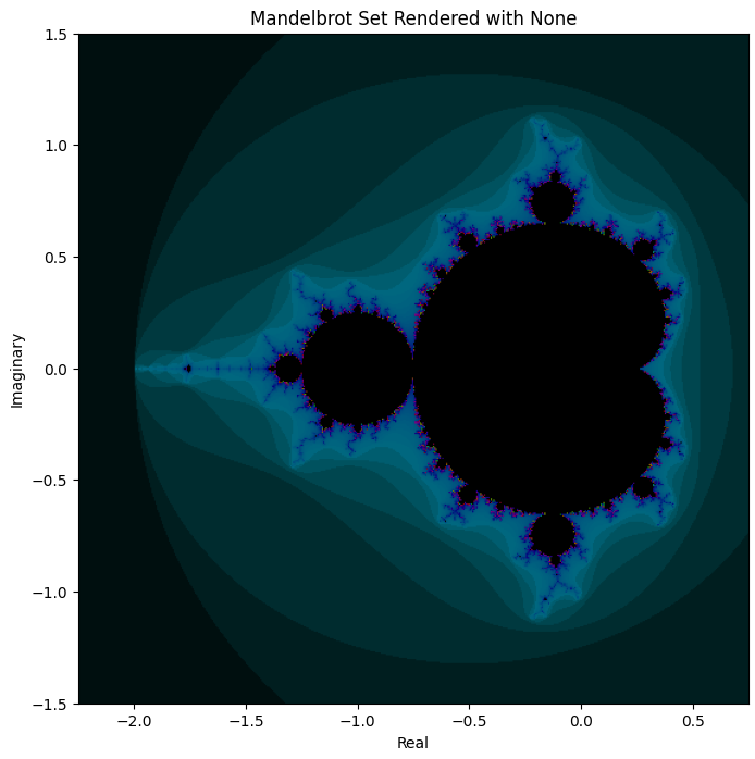
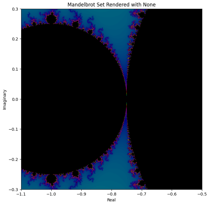
For reference, here’s the actual Mandelbrot, when rendered correctly (with some arbitrary color gradient based on iterations it took to detect divergence):
Rendering it based on Model 0 (no hidden layers), we obtain… something. It’s not very good:
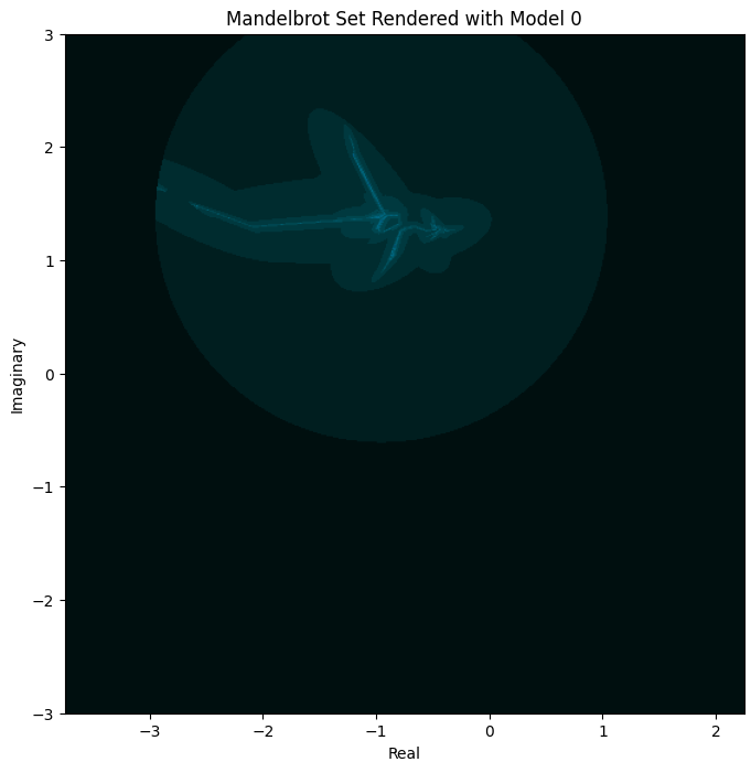
It’s neither Mandelbrot-like, nor even centered around where it’s supposed to be, nor notably “fractal”. Zooming in on the slightly more interesting part:
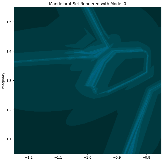
Yeah, not much there. I’ll spare you Model 1 ([10]) which is similarly underwhelming.
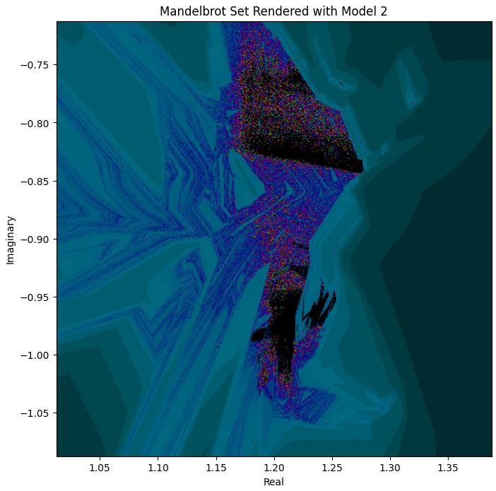
Model 2 ([10, 10]) certainly has something going on:
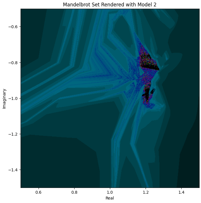
But zooming into the interesting part, it’s closer to repetitive noise than anything fractal-like:
Model 3 ([20, 30, 20]) is actually the first one that has some distant resemblance of Mandelbrot:
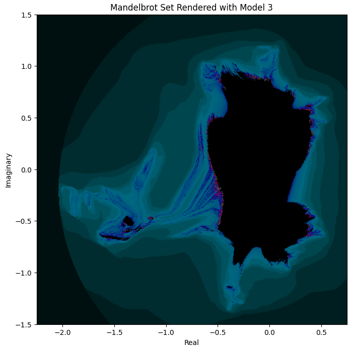
But it’s still extremely far off. I found this surprising, as the visual function comparison in the last section looked very promising for this model.
Now, what about Model 4 ([20, 30, 20] with SiLU)? Based on loss, we saw that using SiLU instead of ReLU made a modest difference, reducing test loss roughly to a third for otherwise same training conditions. But will this make a big difference for what the rendered Mandelbrot looks like?
Have a look:
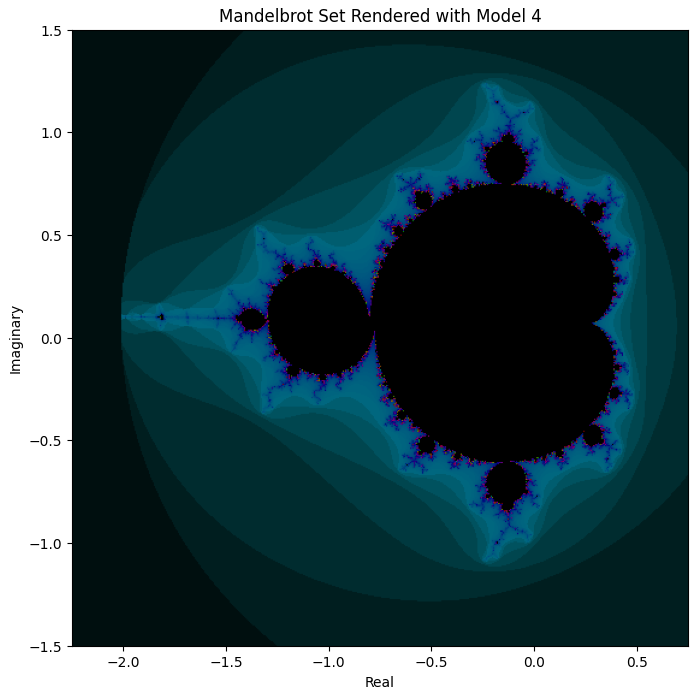
Well, it basically nails it!
And if we zoom in on the middle, the “neck” of the figure:
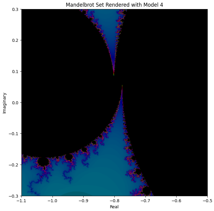
We can see that even zoomed in, a lot of the detail that one would expect is indeed there.
For comparison, here’s what the above viewport should look like:
So we can definitely see some differences, e.g. the one based on Model 4 is much less symmetric—but the basic shapes are all there, just slightly morphed in space.
It’s interesting how Model 3 and Model 4 had test loss values that were not all that far apart (0.34 vs 0.11, respectively), yet their Mandelbrot renderings are worlds apart. Why is that?
I don’t know for sure, but my loose assumption would be something like this:
The difference between model 3 and 4 is that 3 uses ReLU and hence has all these flat, linear patches, whereas model 4 uses SiLU and is much smoother. The way fractals like Mandelbrot are generated is through an iteration of hundreds of steps where we keep multiplying (in the case of Mandelbrot squaring) complex numbers. Multiplication of complex numbers can be interpreted as scaling + rotation. I suppose that in the model 3 case, where much of the space is flat, this iteration just behaves predictably “linear” within these isolated patches of space and doesn’t perform the subtle rotational dance that gives fractals their fractal-ness. So, even though the loss of model 3 and model 4 is not that far apart, model 3 may just lack the “smoothness of space” property that is required for fractals to fractal?
Mandelbrot Training Animation
Finally, I’ve spent some of my compute to visualize the learning process of model 3 and 4 to see what the learned Mandelbrot looks like through the epochs.
Here’s the model 3 architecture (for this animation I trained it a bit longer than for the images above):

It really looks as if there’s a Mandelbrot inside there that’s struggling to push space into its proper shape. Maybe if I’d have let this run for a few hours, we would have gotten somewhere, at least in this zoomed-out view. (Based on my explanation above, I would expect that we’d basically never get a proper fractal that we can zoom into and find “infinite” detail)
It reminds me a bit of a bird struggling to hatch from its egg—and of Ilya Sutskever’s claim that “the models just want to learn”.
And here we have model 4:

It’s interesting how it finds a Mandelbrot-like shape extremely quickly, even while its loss is still much higher than that of the fully trained model 3, and afterwards it’s basically just fine-tuning the spatial proportions.
Importance of Network Initialization
The post carries “gradient descent” in its title, yet so far there was relatively little of that. So let’s leave the fancy visualizations behind and look at some numbers and dimensions.
Firstly, I was interested in the question to what degree the random network initialization determines the ultimate performance of the network. Does an initialized network’s loss determine its performance after n epochs? Is it worth it creating multiple initializations and checking their loss to achieve better results? Or perhaps, one should start with a bunch of random initializations, then trains for m epochs, and continue with the best one from there?
For this, I settled on a simple model architecture (similar to model 2 above: two hidden layers with [10, 10] neurons) and then created 30 models with random initialization.
So, let’s see what their starting test loss distribution looked like:
The initial test loss of the 30 models I set up ranged from roughly 29 to 38 - so some potential for different performance, but not orders of magnitude of difference.
After 10 epochs:
Ranging from roughly 6 to 18.
And after 100:
Ranging from about 1.2 to 3.8.
So there is some difference in performance between the 30 models, but it doesn’t seem that huge and they all keep moving within some relatively narrow band of loss values. I’m not sure if they will all converge to the same lower bound if you train them long enough, but that seems certainly possible based on the above data.
However, based on these histograms, we don’t know which models end up with the lowest loss. So here’s a visualization of the entire process with all 30 models:
It’s hard to make out the details here, but one can certainly see that the order of the models changes a lot. The 3 that started out worst soon caught up (although one of them ends up performing worst again later). And the one that started out best did not stay in first place for long.
Another way to look at this data is to check the correlation of the loss of different models after n vs m epochs. E.g., does the loss after 5 epochs predict the loss after 100 epochs to a strong enough degree that it might be worth training multiple models a bit to then pick the best one for a longer training run?
Probably not—while there is a decent correlation of 0.556, it’s probably small enough that training multiple models a bit will not give you much of an edge vs just taking any model and throwing all your compute at that one. Again, I would be careful to generalize much beyond my toy setup here as with basically all findings, but still interesting to see.
Loss Landscape
Next, I wanted to learn more about the loss landscape. What’s its geometry like? Is it rough? Smooth? Regular? Chaotic? Fractal-esque? Will I find anything unexpected there?
What I ended up doing is this: At different points in time during training, I’d look along the current gradient and scale the learning rate from, say, −10 to 10, and check what loss I’d end up with for the learning rate scaled with these factors. This would then give me a slice of the loss landscape as a R → R graph. What kind of structure do you think this will yield?
For this, I trained a [10, 10, 10] model (don’t ask me why I chose a different one from the earlier experiments—but I don’t think it matters that much) for 45 epochs (45 being arbitrary, I could have equally chosen 5 or 3,000).
And this is the “gradient loss slice” I obtained:
So, again, what do we see here? The x axis shows different scaling factors for the gradient of the model at that point in time. The y axis then shows the relative loss of the network, when the current gradient times the learning rate times the given factor is applied to the model weights (relative to the loss of the model without a change). So, 3 things should be pretty certain and are indeed the case here:
At x = 0, the function should cross 0 (because it’s the relative loss; not changing the network weights at all should not lead to a different loss)
The derivative of this function at x = 0 should be negative (because the gradient as we’re using it here points into a direction of reduced loss)
If the learning rate is remotely well chosen, then in theory the function should have something like a low point around α = 1 – this is not the case here, which I think is because I’m using the Adam optimizer, whereas this gradient function slice is doing regular gradient descent. So the learning rate is chosen pretty well for Adam, but not that well for (S)GD. Hence, this criterion doesn’t fully apply here, and the function’s low point is more towards α = 0.2 or so. But, ehhh, good enough?
Now, what I was surprised by is that this loss landscape is just a parabola (it’s not exactly one—it’s not perfectly symmetrical; but it clearly is very close to one). My initial expectation was to see some way more chaotic landscape. You know, similar to, say, a slice of a mountain on Earth, or something. Or somewhat like a random walk where we only locally know that right in front of us it should descend, but otherwise behaves erratically. But, no, it’s extremely regular and boring. Is this just due to the function we’re approximating? After all, complex number multiplication itself is also pretty regular, smooth and boring. So maybe that’s just the reason?
I went ahead and came up with some cursed and entirely useless function (as a replacement for complex number multiplication, just to see what its loss landscape will look like), optimized purely for the purpose of leading to more interesting geometry:
def interesting_function(a, b, c, d):
  v1 = np.sin(np.pow(np.abs(a),np.abs(b)))
  v2 = np.fmod(d, (b - a))
  v3 = np.min([c, d]) / np.max([c, d])
  v4 = np.fmod(a * b, v3)
  return np.mod(np.abs(v1 * c + (1 - c) * v2), 3), np.mod(np.abs(v3 * v4), 3)
It doesn’t make much sense—I just semi-randomly threw together a bunch of mathematical operators to get some high-frequency irregular behavior out of it.
Visualizing it, I can’t say I’m not happy with how the function turned out:
(The model here clearly struggles to mirror that function, but we can still see it made a bit of progress during training)
So, will this much less regular function also have a much less regular loss landscape? Or will we still just get something parabola-like?
It turns out that even for this function, my gradient slice looks rather boring:
Perhaps it’s just the direction of the gradient that’s boring and regular? Maybe random other directions yield more interesting geometry?
Well, I went ahead and plotted a 2D function, with two (more or less[2]) random directions in weight space, and looked at how a linear combination of them both would affect the loss. And I basically got a bowl:
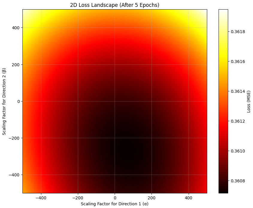
(This now shows absolute, not relative loss, hence the low point does not have a value much below 0)
To be honest, when I went into this experiment, I expected something more in this direction (but with more dimensions):
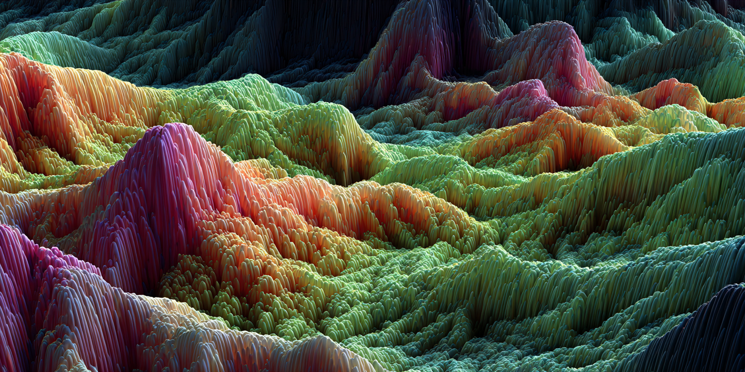
I assumed the loss landscape would be quite erratic and complex, and beyond the local knowledge about “gradient going down here” anything could happen. But it appears that, at least for the two functions I looked at, the loss landscape is indeed very regular and “boring”. If someone has an intuitive understanding for why that should be the case, I’d be very interested to hear it!
Now, I should mention, I’m much less confident in the results of this section than the others, because there are a few things that don’t quite add up for me:
The inconsistency between Adam and regular gradient descent, as mentioned before
That even scaling the gradient by 500x does seemingly not increase the loss that meaningfully
Generally, the whole thing is pretty much vibe-coded, and I can’t claim to have verified every single tiny syllable…

So, ummm… yeah. But, on the other hand: asking Claude Opus 4.1 in a very non-leading way what type of geometry it would expect from the above experiment, it did predict: something that looks like a parabola. So, apparently, this result is not actually surprising, and my expectation of some interesting geometry hiding in this high-dimensional loss landscape was just incorrect.
Parameter Trajectories
I was wondering about one other thing—how do parameters actually move through the high-dimensional parameter space? I could think of at least two options here. As I trained a model (now again on complex number multiplication) and the loss more and more converged towards its lower bound, I could either observe:
The parameters all slowly settling in on their final value
The parameters still moving freely through parameter space, changing a lot even while the loss changes very little (which might make sense if these high-dimensional spaces don’t have “minima” in the classical sense, but rather very high-dimensional “minimum manifolds”, and the parameters kind of drift through/towards these)
Here’s what I found:
These are all weights and biases of a model with hidden layers of sizes [6, 8, 6] that ends up with 154 parameters (4*6 + 6*8 + 8*6 + 6*2 = 132 weights, and 6+8+6+2 = 22 biases).
So, does this look more like option 1 or option 2? Well, hard to say, but perhaps a bit closer to option 1. While most parameters have “settled down” after the first few hundred epochs, clearly some of them are still on a mission, though. I was also a bit surprised how smoothly many of them are moving. The above was with a learning rate of 0.01. Increasing it to 0.03, I got the following:
It still seems to be the case that many parameters are systematically drifting into one direction, albeit now in a more noisy fashion. It gives me “just update all the way bro!” vibes—but perhaps this is a bit of a coordination problem: multiple parameters have to move more or less in unison, and none of them can reasonably update further even though the longer term trajectory is clear. Hence, increasing the learning rate doesn’t appear to help much with arriving at the resulting configuration that much sooner and it just leads to a bunch of back-and-forth now.
Maybe a suitable metaphor would be: when you’re walking through the dark, you’ll take super small steps, even when you know the direction of your destination, as you need to be careful to not trip and fall over. These networks here similarly seem to often move in relatively consistent directions, but need to do so carefully and slowly, as so many parameter need to be coordinated for this to work out.
Returning to a learning rate of 0.01, I then went for a longer training run of 3000 epochs, this time not plotting every single parameter, but instead a few different metrics:
The loss
The “distance traveled” during each epoch, meaning the square root of the sum of squared differences between each parameter’s new value compared to its previous one. So, as the weights move through parameter space, I keep track of the distance covered during each individual epoch. Based on the renderings above, I suspect it should start out large and get smaller and smaller.
The (normalized) dot product between the last and the current update step. This should tell us, roughly, at what points of the training the parameter weights tend to “keep moving in the same direction” (when the dot product is close to 1) vs change directions with each step (when the dot product is closer to 0, or even negative).
The proportion of parameters that have, over the past 100 epochs, drifted by more than 0.05 (a somewhat arbitrary threshold to differentiate “stable” parameters from those that are consistently drifting into a direction)
And we get this mess (starting at epoch 200, so we’re skipping much of the initial chaos):
(Note: the step distance was scaled up by 10x as otherwise it was hard to visually tell it apart from 0)
Some observations:
Even though the parameter trajectories themselves were quite smooth for a 0.01 learning rate, this graph shows that the test loss (blue) behaves quite erratically, perhaps suggestion that 0.01 is even a bit large
The epoch step distance (how far we move through parameter space during each epoch; orange) initially slows down, but seems to settle around roughly 0.015 (0.15 / 10) without notably falling further
However, the proportion of parameters that consistently drift into a direction gets closer and closer to 0 over time, after starting out close to 1. This suggests that while there is still a lot of movement amongst parameters after epoch 1000 or so, it’s less “systematic”, with fewer and fewer parameters following these predefined trajectories
This also matches the dot product graph (red; scatter plot shows actual dot products, whereas the red line shows the moving average of dot products of the last 20 epochs). It starts out > 0 in the first few hundred epochs, suggesting that parameters initially keep moving into very broadly the same direction (or at least: directions from epoch to epoch are somewhat aligned). As we cross 500 epochs though, the dot product becomes predominantly negative, suggesting the parameters doing a lot of “back and forth” movements. This matches the interpretation that many parameters have “settled” and are now hovering around a suitable value.
If the learning rate is indeed somewhat too large, let’s have a look at the same chart but for learning rate 0.001. Note that the out-of-view epochs (the first 200) still use learning rate 0.01, to get to the same visible starting point (and to get the test loss to roughly 1 so the chart looks nice with all 4 lines sharing the same y-axis).
Indeed, the test loss is much less volatile here—and even reaches a lower loss than before (~0.2 after 3000 epochs, compared to ~0.23 with the previous higher learning rate). Additionally it appears that the dot product is now (for the observed 3000 epochs) consistently positive, suggesting that parameters are moving much more regularly/predictably in slowly-changing directions rather than back-and-forth. I would suppose that the dot product eventually drops below 0 here as well. Alright, let’s test that as well, and then we call it a day.
Here we go, 12k epochs instead of 3k:
Interestingly, while the dot product now does generally drop below 0 after around 5000 epochs, it occasionally jumps back up above 0 every now and then for a hundred epochs at a time or so. So it appears that interesting things are still going on to some degree even after 10k+ epochs.
Wrapping Up
What should we take away from all of this? It’s a bit hard to say, given that it’s unclear to what degree my findings here generalize beyond the simple toy model I’ve been investigating.
But if I had to summarize some loosely acquired beliefs that I took away from this:
My complex number multiplication networks seemed to not do very “interesting” things, but merely did some piece-wise approximation of the function. Maybe this is very common for neural networks? But then again, maybe “piece-wise approximation” of high-dimensional learned latent spaces just is way more interesting than it sounds. Also, Neel Nanda’s modular addition paper appears to suggest a network learning a more interesting algorithm eventually for that particular scenario, so I guess this does happen after all, given the right circumstances.
This is pretty specific to my particular use case here and not a general ML insight, but it was certainly interesting to see that the generated fractals benefited much more from a smooth activation function than from low loss in the learned function. Perhaps a relevant insight to derive from this is something like: loss is not everything, and there can be situations where the shape of the resulting function is more important than the mere loss.
The longest training run I’ve had was ~12 minutes long, but in all these training runs, I never encountered a loss actually fully plateauing—it always still seemed to drop very slowly. So it was surprisingly hard for me, even given this very simple function, to encounter anything like a real lower bound for the loss in any of these networks, although I’d assume that such lower bounds must exist, and these networks can’t just get arbitrarily close to 0 loss.
I didn’t find much evidence of the random initialization of the network mattering that much. While there was some correlation between initial test loss and test loss after n epochs, this correlation was likely too weak to be exploitable in any meaningful way. That being said, there probably are cases where you can end up being unlucky with an initialization, e.g. I remember this being mentioned somewhere in this video.
For the functions I looked at, the loss landscape looked surprisingly regular/smooth, not to say boring. Same for the parameter trajectories: after a lot of movement in early epochs, most parameters settle down for longer time frames, and those that don’t, mostly happen to move pretty consistently in one direction. Increasing the learning rate doesn’t help much though to speed these predictable trends up: even though many parameters predictably trend into one direction, it appears they need to move “cautiously” in sync with other parameters, making it difficult for them to reach their eventual destination more quickly.
That all being said, I’m sure there are many things I got wrong in this post, from parts of the implementation to my interpretations of the results. Maybe even some of the questions I’ve been asking are misguided. So, if anyone actually took the time to read (parts of) this post, please feel very free to correct any misconceptions and errors you encounter. I’d also be happy about further interesting questions getting raised that I failed to think of which would be worth exploring.
I hope this exploration was interesting enough and maybe even contained some novel insights. Thanks for reading!
I like the spirit of this work but it would benefit a lot from a more in depth review of the existing literature and methodologies. some examples (non exhaustive)
the piecewise approximation thing is a pretty widely accepted opinion in ML
visualizing the loss landscape as a plane between three points in model space is pretty common in the field and often the landscape is a lot more nontrivial.
a factor of 3 loss difference is huge! if you want to claim that smooth actfn is better beyond what’s explained by the loss, you need to compare two models with the same loss but different actfn.
the post just hand waves away the difference between SGD and Adam. this is an important difference! Adam tries to take ~constant sized steps along each axis direction.
local approximation of the loss landscape as approximately quadratic is pretty widely accepted; generally people look at the eigenvalues of the Hessian to try to understand the local shape of the loss landscape.
scaling the gradient 500x is less impactful than it sounds like because the changes to the gradient scale are way less important than you’d expect because they get multiplied out by (1-beta2), this is unlike SGD where gradient scaling is equivalent to LR scaling.
learning rate decay is an important part of real training that substantially affects many conclusions
to compare models, if possible generally you want to train to the L(D) regime (loss has stopped improving at all), or pick some principled criterion for stopping early compute-optinally (L(C))
I made a fairer comparison now. Training model 4 (same architecture as model 3, but SiLU instead of ReLU) for only 30 epochs, it achieves a test loss of 0.3435, slightly above the 0.3403 of model 3. Taking these two models to render Mandelbrot, I get these results:
Model 3 (as we’ve seen in the post):
Model 4 with slightly worse test loss than Model 3:
And zooming in a bit to see the fractal details of Model 4:
So I’d say the observation holds—the huge difference between rendered Mandelbrot quality for some reason does not depend so much on the loss here. Even for (roughly) identical loss, they are worlds apart. So my take is that the smoothness of the SiLU activation function somehow enables the fractal iteration to work out much better (but not really sure how else to test this vague assumption).
In fact, even after only 10 epochs and a test loss of >1.2, model 4 already produces something that clearly resembles Mandelbrot, which model 3 failed to achieve even after 100s of epochs:
Thanks for the comment!
This is definitely not wrong. Probably depends a bit on what one sees as the goal here though—in my case, after weeks of readings and exercises, I was in dire need of basically just playing around with things more freely. So it was less about “how can I create the most valuable possible lesswrong post”, and more “I’m going to do this thing anyway, and perhaps documenting the project in a lesswrong post is better than not doing so”. I’m not totally confident about that though.
Thanks a lot for the list! Very interesting points that give me some ideas of where to go next.
Sounds like good news to me! Certainly not the worst thing if the thing I found happens to be widely accepted. (also makes sense now that in both cases, Claude predicted these outcomes (even though I only asked it after getting to these findings—but asked as if I didn’t know what to expect) - I guess it was less about Claude being very smart then and more about these things being relatively well established anyway)
Fair point! My coverage of that in the post wasn’t great. What I didn’t mention there is that during the rendering of the two videos of model3 and model4 “learning Mandelbrot”, model4 had the shape (including “fractal depth”) down way before even getting close to the loss that model3 had at the end. So even with much lower loss, the ReLU Mandelbrot looked much worse than that of SiLU. But I’ll look into that again and make a proper comparison.
One addition: I’ve been privately informed that another interesting thing to look at would be a visualization of C² (rather than only multiplication of a constant complex number with other complex numbers, see Visualizing Learned Functions section).
So I did that. For instance, here’s the square visualization of model2 (the one with [10, 10] hidden neurons):
Again, we see some clear parallel between reality and the model, i.e. colors end up in roughly the right places, but it’s clearly quite a bit off anyway. We also still see a lot of “linearity”, i.e. straight lines in the model predictions as well as the diff heatmap, but this linearity is now seemingly only occurring in “radial” form, towards the center.
Model 0 and 1 look similar / worse. Model 3 ([20, 30, 20] hidden neurons) gets much closer despite still using ReLU:
And model 4 (same but with SiLU), expectedly, does even better:
But ultimately, we see the same pattern of “the larger the model, the more accurate, and SiLU works better than ReLU” again, without any obvious qualitative difference between SiLU and ReLU—so I don’t think these renderings give any direct hint of SiLU performing that much better for actual fractal renderings than ReLU.
If I can ask, just as a matter of practicality that I might be interested in because I’ve been looking at ARENA myself—at what point did you find that it was basically impossible to go forward with your own hardware, and what did you use to go past that point if you reached it?
You mean in ARENA or with this complex number multiplication project? In both cases I was just using Google Colab (i.e. cloud compute) anyway. It probably would have worked in the free tier, but I did buy $10 worth of credits to speed things up a bit, as in the free tier I was occasionally downgraded to a CPU runtime after running the notebook for too long throughout a day. So I never tried this on my own hardware.
For this project, I’m pretty sure it would have worked completely fine locally. For ARENA, I’m not entirely sure, but would expect so too (and I think many people do work through it locally on their device with their own hardware). I think the longest training run I’ve encountered took something like 30 minutes on a T4 GPU in Colab, IIRC. According to Claude, consumer GPUs should be able to run that in a similar order of magnitude. Whereas if you only have some mid-range laptop without a proper graphics card, Claude expects a 10-50x slowdown, so that might become rather impractical for some of the ARENA exercises, I suppose.
All right, thanks! I wasn’t really aware of Colab’s free tier extents so it’s good to know there’s something of an intermediate stage between using my laptop and paying for compute. Also an easier interface than having to e.g. use AWS… personally I’d also be ok with just SSH’ing into a remote machine and working there but I’m not sure if anyone offers something like that.
I have a gaming laptop, so a decently powerful GPU but it obviously still isn’t as beefy as what you can rent from these compute services.
One more addition: Based on @leogao’s comment, I went a bit beyond the “visualize loss landscape based on gradient” approach, and did the following: I trained 3 models of identical architecture (all using [20, 30, 20] hidden neurons with ReLU) for 100 epochs and then had a look at the loss landscape in the “interpolation space” between these three models (such that model1 would be at (0,0), model2 at (1,0), model3 at (0,1), and the rest just linearly interpolating between their weights). I visualized the log of the loss at each point. My expectation was to get clear minima at (0,0), (1,0) and (0,1), where the trained models are placed, and something elevated between them. And indeed:
Otherwise the landscape does look pretty smooth and boring again.