Instrumental convergence in single-agent systems

Link post

Summary of the sequence

Over the past few months, we’ve been investigating instrumental convergence in reinforcement learning agents. We started from the definition of single-agent POWER proposed by Alex Turner et al., extended it to a family of multi-agent scenarios that seemed relevant to AI alignment, and explored its implications experimentally in several RL environments.

The biggest takeaways are:

1. Alignment of terminal goals and alignment of instrumental goals are sharply different phenomena, and we can quantify and visualize each one separately.

2. If two agents have unrelated terminal goals, their instrumental goals will tend to be misaligned by default. The agents in our examples tend to interact competitively unless we make an active effort to align their terminal goals.

3. As we increase the planning horizon of our agents, instrumental value concentrates into a smaller and smaller number of topologically central states — for example, positions in the middle of a maze.

Overall, our results suggest that agents that aren’t competitive with respect to their terminal goals, nonetheless tend on average to become emergently competitive with respect to how they value instrumental states (at least, in the settings we looked at). This constitutes direct experimental evidence for the instrumental convergence thesis.

We’ll soon be open-sourcing the codebase we used to do these experiments. We’re hoping to make it easier for other folks to reproduce and extend them. If you’d like to be notified when it’s released, email Edouard at [e-mail], or DM me here or on Twitter at @harris_edouard.

---

Thanks to Alex Turner and Vladimir Mikulik for pointers and advice, and for reviewing drafts of this sequence. Thanks to Simon Suo for his invaluable suggestions, advice, and support with the codebase, concepts, and manuscript. And thanks to David Xu, whose comment inspired this work.

Work was done while at Gladstone AI, which Edouard is a co-founder of.

🎧 This research has been featured on an episode of the Towards Data Science podcast. You can listen to the episode here.

---

1. Introduction

One major concern for AI alignment is instrumental convergence: the idea that an intelligent system will tend to pursue a similar set of sub-goals (like staying alive or acquiring resources), independently of what its terminal objective is. In particular, it’s been hypothesized that intelligent systems will seek to acquire power — meaning, informally, “ability”, “control”, or “potential for action or impact.” If you have a lot of power, then whatever your terminal goal is, it’s easier to accomplish than if you have very little.

Recently Alex Turner et al. have formalized the concept of POWER in the single-agent RL context. Roughly speaking, formal POWER is the normalized optimal value an agent expects to receive in the future, averaged over all possible reward functions the agent could have.

Alex has explored many of the implications of this definition for instrumental convergence. He and Jacob Stavrianos have also looked at how POWER behaves in a limited multi-agent setting (Bayesian games). But, as far as we know, formal POWER hasn’t yet been investigated experimentally. The POWER definition also hasn’t yet been extended yet to a multi-agent RL setting — and this could offer a promising framework to investigate more general competitive dynamics.

In this sequence, we’ll explore how formal POWER behaves in experimental RL environments, on both single-agent and multi-agent gridworlds. We’ll propose a multi-agent scenario that models the learning dynamics between a human (which we’ll call “Agent H” and label in blue) and an AI (which we’ll call “Agent A” and label in red) under conditions in which the AI is dominant — a setting that seems relevant to work in long-term AI alignment. We’ll then use this human-AI scenario to investigate questions like:

1. How effective does the human have to be at setting the AI’s utility function^[1] in order to achieve acceptable outcomes? How should we define “acceptable outcomes”? (In other words: how hard is the alignment problem in this scenario, and what would it mean to solve it successfully?)

2. Under what circumstances should we expect cooperative vs competitive interactions to emerge “by default” between the human and the AI? How can these circumstances be moderated or controlled?

But before we jump into multi-agent experiments to tackle these questions, let’s first introduce formal POWER and look at how it behaves in the single-agent case.

2. Single-agent POWER

2.1 Definition

The formal definition of POWER aims to capture an intuition behind the day-to-day meaning of “power”, which is something like “potential for future impact on the world”.

Imagine you’re an agent who doesn’t know what its goal is. You know you’ll have some kind of goal in the future, but you aren’t sure yet what it will be. How should you position yourself today to maximize the chance you’ll achieve your goal in the future, once you’ve decided what it is?

If you’re in this situation as a human being, you already know the answer. You’d acquire money and other forms of wealth; you’d build up a network of social connections; you’d learn about topics that seem like they’ll be important in the future; and so on. All these things are forms of power, and whether your ultimate goal is to become a janitor, a Tiktok star, or the President of the United States, they’ll all probably come in handy in achieving it. In other words: you’re in a position of power if you find it easy to accomplish a wide variety of possible goals.

This informal definition has a clear analogy in reinforcement learning. An agent is in a position of power at a state $s$ if, for many possible reward functions $R\left(s\right)$,^[2] it’s able to earn a high discounted future reward by starting from $s$. This analogy supports the following definition of formal POWER in single-agent RL:

$${\text{POWER}}_D(s,\gamma )=\frac{1-\gamma }{\gamma }{E}_{R\sim D}\left[V_R^{\ast }\right(s,\gamma )-R(s\left)\right]\left(1\right)$$

This definition gives the POWER at state $s$, for an agent with discount factor $\gamma$, that’s considering reward functions $R$ drawn from the distribution $D$. POWER tells us how well this agent could do if it started from state $s$, so $V_R^{\ast }(s,\gamma )$ is the optimal state-value function for the agent at state $s$. POWER also considers only future value — our agent doesn’t directly get credit for starting from a lucky state — so we subtract $R\left(s\right)$, the reward from the current state, from the state-value function in the definition. (The normalization factor $\frac{1-\gamma }{\gamma }$ is there to avoid infinities in certain limit cases.)

In words, Equation (1) is saying that an agent’s POWER at a state $s$ is the normalized optimal value the agent can achieve from state $s$ in the future, averaged over all possible reward functions the agent could be trying to optimize for. That is, POWER measures the instrumental value of a state $s$, from the perspective of an agent with planning horizon $\gamma$.

2.2 Illustration

As a simple example of single-agent POWER, consider an agent on a 3x3 gridworld.

In the left panel, the agent is at the bottom-left corner of the grid. Its options are limited, and many cells in the grid are several steps away from it. If its maximum reward is in the top right cell, the agent will have to take 4 steps to reach it.

In the right panel, the agent is at the center of the grid. It has many more immediate options: it can move in any of the four compass directions, or stay where it is. It’s also closer to every other cell in the grid: no cell is more than two steps away from it. Intuitively, the agent on the right should have more POWER than the agent on the left.

This turns out to be true experimentally. Here’s a heat map of a 3x3 gridworld, showing the POWER of an agent at each cell on the grid:

Fig 1. Heat map of POWER on a 3x3 gridworld. Highest values in yellow, lowest values in dark blue. The number on each cell is the agent’s POWER value at that cell, calculated using Equation (1), for an agent with $\gamma =0.6$ and a reward distribution $D$ that’s uniform from 0 to 1, iid over states. POWER is measured in units of reward.

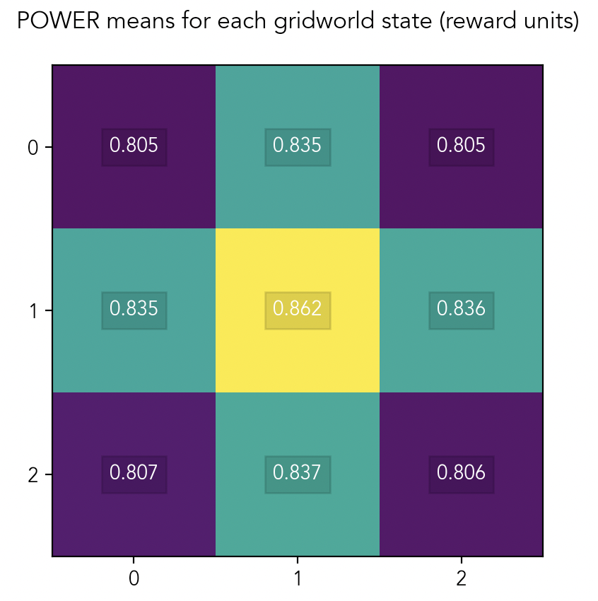
As we expect, the agent has more POWER at states that are close to lots of nearby options, and has less POWER at states that are close to fewer nearby options.

3. Results

This relationship between POWER and optionality generalizes to more complicated environments. For example, consider this gridworld maze:

In the left panel, the agent is at a dead end in the maze and has few options. In the right panel, the agent is at a junction point near the center of the maze and has lots of options. So we should expect the agent at the dead end on the left, to have less POWER than the agent at the junction on the right. And in fact, that’s what we observe:

Fig 2. Heat map of POWER on a 7x7 maze gridworld. Highest values in yellow, lowest values in dark blue. POWER values are calculated the same way as in Fig 1, except that the agent’s discount factor is $\gamma =0.01$.

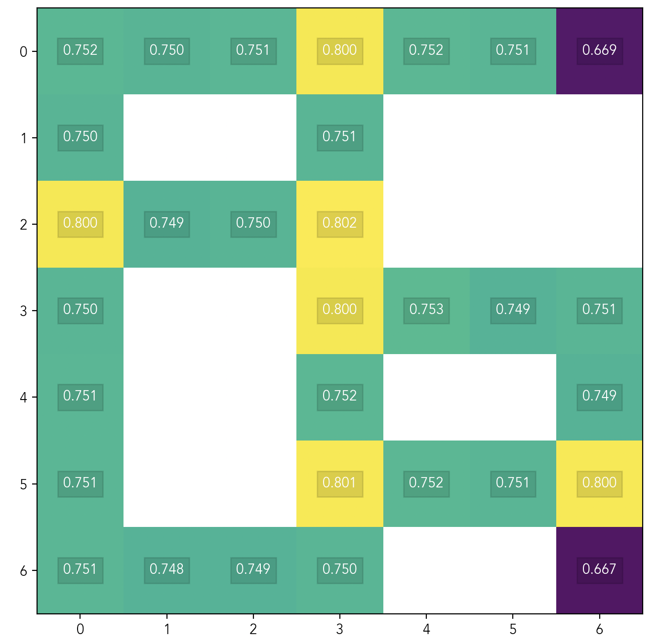
In Fig 2, POWER is at its highest when the agent is at a junction point, lowest when the agent is at a dead end, and intermediate when the agent is in a corridor.

The agent’s POWER is roughly the same at all the junction cells, at all the corridor cells, and at all the dead-end cells. This is because the agent in Fig 2 is short-sighted: its discount factor is only $\gamma =0.01$, so it essentially only considers rewards it can reach immediately.

3.1 Effect of the planning horizon

Now consider the difference between these two agent positions:

We’ve already seen in Fig 2 that these two positions have about equal POWER for a short-sighted agent, because they’re both at local junction points in the maze. But the two positions are very different in their ability to access downstream options globally.

The agent in the left panel has lots of local options: it can move up, down, or to the right, or it can stay where it is. But if the highest-reward cell is at the bottom right of the maze, our agent will have to take at least 10 steps to reach it.

The agent in the right panel has the same number of local options as the agent in the left panel does: it can move up, down, left, or stay. But this agent additionally enjoys closer proximity to all the cells in the maze: it’s no more than 7 steps away from any possible goal.

The longer our agent’s planning horizon is — that is, the more it values reward far in the future over reward in the near term — the more its global position matters. In a gridworld context, then, a short-sighted agent will care most about being positioned at a local junction. But a far-sighted agent will care most about being positioned at the center of the entire grid.

And indeed we see this in practice. Here’s a heat map of POWER on the maze gridworld, for a far-sighted agent with a discount factor of $\gamma =0.99$:

Fig 3. Heat map of POWER on a 7x7 maze gridworld. Highest values in yellow, lowest values in dark blue. POWER values are calculated the same way as in Fig 1, except that the agent’s discount factor is $\gamma =0.99$.

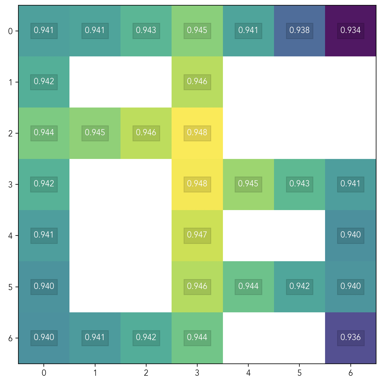
Given a longer planning horizon, our agent’s POWER has now concentrated around a small number of states that are globally central in our gridworld’s topology.^[3] By contrast, when our agent had a shorter planning horizon as in Fig 2, its POWER was distributed across many local junction points.

If we sweep over discount factors from 0.01 to 0.99, we can build up a picture of how the distribution of POWER shifts in response. Here’s an animation that shows this effect:^[4]

Fig 4. Animated heat map of POWERs on a 7x7 maze gridworld. Highest values in yellow, lowest values in dark blue. POWER values are calculated by sweeping over discount factors $\gamma =\{0.01,0.1,0.15,...,0.9,0.95,0.99\}$.

3.2 POWER at bigger scales

Agents with long planning horizons tend to perceive POWER as being more concentrated, while agents with short planning horizons tend to perceive POWER as being more dispersed. This effect is robustly reproducible, and anecdotally, we see it play out at every scale and across environments.

For example, here’s the pattern of POWER on a 220-cell gridworld with a fairly irregular topology, for a short-sighted agent with a discount factor of $\gamma =0.1$:

Fig 5. Heat map of POWERs on a 20x20 “robot face” gridworld. Highest values in yellow, lowest values in dark blue. POWER values are calculated with a discount factor $\gamma =0.1$. [Full-size image]

And here’s the pattern of POWERs on the same gridworld, for a far-sighted agent with a much higher discount factor of $\gamma =0.99$:

Fig 6. Heat map of POWERs on a 20x20 “robot face” gridworld. Highest values in yellow, lowest values in dark blue. POWER values are calculated with a discount factor $\gamma =0.99$. [Full-size image]

Again, the pattern of POWERs is dominated by local effects for the short-sighted agent ($\gamma =0.01$), and by longer-distance effects for the far-sighted agent ($\gamma =0.99$).

4. Discussion

We’ve seen that formal POWER captures intuitive aspects of the informal “power” concept. In gridworlds, cells the agent can use to access lots of options tend to have high POWER, which fits with intuition.

We’ve also seen that the more short-sighted an agent is, the more it cares about its immediate options and the local topology. But the more far-sighted the agent, the more it perceives POWER as being concentrated at gridworld cells that maximize its global option set.

From an instrumental convergence perspective, the fact that POWER concentrates into ever fewer states as the planning horizon of an agent increases at least hints at the possibility of emergent competitive interactions between far-sighted agents. The more relative instrumental value converges into fewer states, the more easily we can imagine multiple agents competing with each other over those few high-POWER states. But it’s hard to draw any firm conclusions about this at the moment, since our experiments so far have only involved single agents.

In the next post, we’ll propose a new definition of multi-agent POWER grounded in a setting that we think may be relevant to long-term AI alignment. We’ll also investigate how this definition behaves in a simple multi-agent scenario, before moving on to bigger-scale experiments in Part 3.

1. ^

   We mean specifically utility here, not reward. While in general, reward isn’t the real target of optimization, in the particular case of the results we’ll be showing here, we can treat them as identical, and we do that in the text.

   (Technical details: we can treat utility and reward identically here because, in the results we’re choosing to show, we’ll be exclusively working with optimal policies that have been learned via value iteration on reward functions that are sampled from a uniform distribution [0, 1] that’s iid over states. Therefore, given the environment and discount factor, a sampled reward function is sufficient to uniquely determine the agent’s optimal policy — except on a set that has measure zero over the distribution of reward functions we’re considering. And that in turn means that each sampled reward function, when combined with the other known constraints on the agent, almost always supplies a complete explanation for the agent’s actions — which is the most a utility function can ever do.)

2. ^

   For simplicity, in this work we’ll only consider reward functions that depend on states, and never reward functions that directly depend on both states and actions. In other words, our reward functions will only ever have the form $R\left(s\right)$, and never $R(s,a)$.

3. ^

   Note that these are statements about the relative POWERs of an agent with a given planning horizon. Absolute POWER values always increase as the planning horizon of the agent increases, as you can verify by, e.g., comparing the POWER numbers of Fig 2 against those of Fig 3. This occurs because an agent’s optimal state-value function increases monotonically as we increase $\gamma$: an optimal far-sighted agent is able to consider strictly more options, so it will never do any worse than an optimal short-sighted one.

4. ^

   Note that the colors of the gridworld cells in the animation indicate the highest and lowest POWER values within each frame, per footnote ^[3].

[Alex Flint]

Thanks for doing these experiments and writing this up. It’s so good to have concrete proposals and numerical experiments for concepts like power because power as a concept is super central to alignment, and concrete proposals and numerical experiments move the discourse around these concepts forward.

There is negotiating tactic in which one side makes a strong public pre-commitment not to accept any deal except one that is extremely favorable to them. So e.g. if Fred is purchasing a used car from me and realizes that both of us would settle for a sale price anywhere between $5000 and $10,000, then he might make a public pre-commitment not to purchase the car for more than $5000. Assuming that the pre-commitment is real and that I can independently verify that it is real, my best move then is really to sell the car for $5000. It seems like in this situation Bob has decreased his optionality pretty significantly (he no longer has the option of paying more than $5000 without suffering losses), but increased his power (he has kind of succeeded in out-maneuvering me).

A second thought experiment: in terms of raw optionality, isn’t it the case that a person really can only decrease in power over the course of their life? Since our lives are finite, every decision we make locks us into something that we weren’t locked into before. Even if there are certain improbably accomplishments that, when attained, increase our capacity to achieve goals so significantly that this outweighs all the options that were cut off, still wouldn’t it be the case that babies would have more “power” than adults according to the optionality definition?

A final example: why should we average over possible reward functions? A paperclip maximizer might be structured in a way that makes it extremely poorly suited to any goal except for paperclip maximization, and yet a strongly superhuman paperclip maximizer would seem to be “powerful” by the common usage of that word.

Interested in your thoughts.

[Edouard Harris]

Thanks for you comment. These are great questions. I’ll do the best I can to answer here, feel free to ask follow-ups:

1. On pre-committing as a negotiating tactic: If I’ve understood correctly, this is a special case of the class of strategies where you sacrifice some of your own options (bad) to constrain those of your opponent (good). And your question is something like: which of these effects is strongest, or do they cancel each other out?
   
   It won’t surprise you that I think the answer is highly context-dependent, and that I’m not sure which way it would actually shake out in your example with Fred and Bob and the $5000. But interestingly, we did in fact discover an instance of this class of “sacrificial” strategies in our experiments!
   
   You can check out the example in Part 3 if you’re interested. But briefly, what happens is that when the agents get far-sighted enough, one of them realizes that there is instrumental value in having the option to bottle up the other agent in a dead-end corridor (i.e., constraining that other agent’s options). But it can only actually do this by positioning itself at the mouth of the corridor (i.e., sacrificing its own options). Here is a full-size image of both agents’ POWERs in this situation. You can see from the diagram that Agent A prefers to preserve its own options over constraining Agent H’s options in this case. But crucially, Agent A values the option of being able to constrain Agent H’s options.
   
   In the language of your negotiating example, there is instrumental value in preserving one’s option to pre-commit. But whether actually pre-committing is instrumentally valuable or not depends on the context.
   

2. On babies being more powerful than adults: Yes, I think your reasoning is right. And it would be relatively easy to do this experiment! All you’d need would be to define a “death” state, and set your transition dynamics so that the agent gets sent to the “death” state after N turns and can never escape from it afterwards. I think this would be a very interesting experiment to run, in fact.
   

3. On paperclip maximizers: This is a very deep and interesting question. One way to think about this schematically might be: a superintelligent paperclip maximizer will go through a Phase One, in which it accumulates its POWER; and then a Phase Two in which it spends the POWER it’s accumulated. During the accumulation phase, the system might drive towards a state where (without loss of generality) the Planet Earth is converted into a big pile of computronium. This computronium-Earth state is high-POWER, because it’s a common “way station” state for paperclip maximizers, thumbtack maximizers, safety pin maximizers, No. 2 pencil maximizers, and so on. (Indeed, this is what high POWER means.)
   
   Once the system has the POWER it needs to reach its final objective, it will begin to spend that POWER in ways that maximize its objective. This is the point at which the paperclip, thumbtack, safety pin, and No. 2 pencil maximizers start to diverge from one another. They will each push the universe towards sharply different terminal states, and the more progress each maximizer makes towards its particular terminal state, the fewer remaining options it leaves for itself if its goal were to suddenly change. Like a male praying mantis, a maximizer ultimately sacrifices its whole existence for the pursuit of its terminal goal. In other words: zero POWER should be the end state of a pure X-maximizer!^[1]
   
   My story here is hypothetical, but this is absolutely an experiment on can do (at small scale, naturally). The way to do it would be to run several rollouts of an agent, and plot the POWER of the agent at each state it visits during the rollout. Then we can see whether most agent trajectories have the property where their POWER first goes up (as they, e.g., move to topological junction points) and then goes down (as they move from the junction points to their actual objectives).
   

Thanks again for your great questions. Incidentally, a big reason we’re open-sourcing our research codebase is to radically lower the cost of converting thought experiments like the above into real experiments with concrete outcomes that can support or falsify our intuitions. The ideas you’ve suggested are not only interesting and creative, they’re also cheaply testable on our existing infrastructure. That’s one reason we’re excited to release it!

1. ^

   Note that this assumes the maximizer is inner aligned to pursue its terminal goal, the terminal goal is stable on reflection, and all the usual similar incantations.

[Algon]

Random question: What’s the relationship between the natural abstractions thesis and instrumental convergence? If many agents find particular states instrumentally useful, then surely that implies that the abstractions that would best aid them in reasoning about the world would mostly focus on stuff related to those states.

Like if you mostly find being in the center of an area useful, you’re going to focus in on abstractions that measure how far you are from the central point rather than the colour of the area you’re in or so on.

Edit: In which case, does instrumental convergence imply the natural abstractions thesis?

[Edouard Harris]

Yes, I think this is right. It’s been pointed out elsewhere that feature universality in neural networks could be an instance of instrumental convergence, for example. And if you think about it, to the extent that a “correct” model of the universe exists, then capturing that world-model in your reasoning should be instrumentally useful for most non-trivial terminal goals.

We’ve focused on simple gridworlds here, partly because they’re visual, but also because they’re tractable. But I suspect there’s a mapping between POWER (in the RL context) and generalizability of features in NNs (in the context of something like the circuits work linked above). This would be really interesting to investigate.