Conditional Independence, and Naive Bayes
Previously I spoke of mutual information between X and Y, I(X;Y), which is the difference between the entropy of the joint probability distribution, H(X,Y) and the entropies of the marginal distributions, H(X) + H(Y).
I gave the example of a variable X, having eight states 1..8 which are all equally probable if we have not yet encountered any evidence; and a variable Y, with states 1..4, which are all equally probable if we have not yet encountered any evidence. Then if we calculate the marginal entropies H(X) and H(Y), we will find that X has 3 bits of entropy, and Y has 2 bits.
However, we also know that X and Y are both even or both odd; and this is all we know about the relation between them. So for the joint distribution (X,Y) there are only 16 possible states, all equally probable, for a joint entropy of 4 bits. This is a 1-bit entropy defect, compared to 5 bits of entropy if X and Y were independent. This entropy defect is the mutual information—the information that X tells us about Y, or vice versa, so that we are not as uncertain about one after having learned the other.
Suppose, however, that there exists a third variable Z. Z has two states, “even” and “odd”, perfectly correlated to the evenness or oddness of (X,Y). In fact, we’ll suppose that Z is just the question “Are X and Y even or odd?”
If we have no evidence about X and Y, then Z itself necessarily has 1 bit of entropy on the information given. There is 1 bit of mutual information between Z and X, and 1 bit of mutual information between Z and Y. And, as previously noted, 1 bit of mutual information between X and Y. So how much entropy for the whole system (X,Y,Z)? You might naively expect that
H(X,Y,Z) = H(X) + H(Y) + H(Z) - I(X;Z) - I(Z;Y) - I(X;Y)
but this turns out not to be the case.
The joint system (X,Y,Z) only has 16 possible states—since Z is just the question “Are X & Y even or odd?”—so H(X,Y,Z) = 4 bits.
But if you calculate the formula just given, you get
(3 + 2 + 1 − 1 − 1 − 1)bits = 3 bits = WRONG!
Why? Because if you have the mutual information between X and Z, and the mutual information between Z and Y, that may include some of the same mutual information that we’ll calculate exists between X and Y. In this case, for example, knowing that X is even tells us that Z is even, and knowing that Z is even tells us that Y is even, but this is the same information that X would tell us about Y. We double-counted some of our knowledge, and so came up with too little entropy.
The correct formula is (I believe):
H(X,Y,Z) = H(X) + H(Y) + H(Z) - I(X;Z) - I(Z;Y) - I(X;Y | Z)
Here the last term, I(X;Y | Z), means, “the information that X tells us about Y, given that we already know Z”. In this case, X doesn’t tell us anything about Y, given that we already know Z, so the term comes out as zero—and the equation gives the correct answer. There, isn’t that nice?
“No,” you correctly reply, “for you have not told me how to calculate I(X;Y|Z), only given me a verbal argument that it ought to be zero.”
We calculate I(X;Y|Z) just the way you would expect. I(X;Y) = H(X) + H(Y) - H(X,Y), so:
I(X;Y|Z) = H(X|Z) + H(Y|Z) - H(X,Y|Z)
And now, I suppose, you want to know how to calculate the conditional entropy? Well, the original formula for the entropy is:
H(S) = Sum i: p(Si)*-log2(p(Si))
If we then learned a new fact Z0, our remaining uncertainty about S would be:
H(S|Z0) = Sum i: p(Si|Z0)*-log2(p(Si|Z0))
So if we’re going to learn a new fact Z, but we don’t know which Z yet, then, on average, we expect to be around this uncertain of S afterward:
H(S|Z) = Sum j: (p(Zj) * Sum i: p(Si|Zj)*-log2(p(Si|Zj)))
And that’s how one calculates conditional entropies; from which, in turn, we can get the conditional mutual information.
There are all sorts of ancillary theorems here, like:
H(X|Y) = H(X,Y) - H(Y)
and
if I(X;Z) = 0 and I(Y;X|Z) = 0 then I(X;Y) = 0
but I’m not going to go into those.
“But,” you ask, “what does this have to do with the nature of words and their hidden Bayesian structure?”
I am just so unspeakably glad that you asked that question, because I was planning to tell you whether you liked it or not. But first there are a couple more preliminaries.
You will remember—yes, you will remember—that there is a duality between mutual information and Bayesian evidence. Mutual information is positive if and only if the probability of at least some joint events P(x, y) does not equal the product of the probabilities of the separate events P(x)*P(y). This, in turn, is exactly equivalent to the condition that Bayesian evidence exists between x and y:
I(X;Y) > 0 =>
P(x,y) != P(x)*P(y)
P(x,y) / P(y) != P(x)
P(x|y) != P(x)
If you’re conditioning on Z, you just adjust the whole derivation accordingly:
I(X;Y | Z) > 0 =>
P(x,y|z) != P(x|z)*P(y|z)
P(x,y|z) / P(y|z) != P(x|z)
(P(x,y,z) / P(z)) / (P(y, z) / P(z)) != P(x|z)
P(x,y,z) / P(y,z) != P(x|z)
P(x|y,z) != P(x|z)
Which last line reads “Even knowing Z, learning Y still changes our beliefs about X.”
Conversely, as in our original case of Z being “even” or “odd”, Z screens off X from Y—that is, if we know that Z is “even”, learning that Y is in state 4 tells us nothing more about whether X is 2, 4, 6, or 8. Or if we know that Z is “odd”, then learning that X is 5 tells us nothing more about whether Y is 1 or 3. Learning Z has rendered X and Y conditionally independent.
Conditional independence is a hugely important concept in probability theory—to cite just one example, without conditional independence, the universe would have no structure.
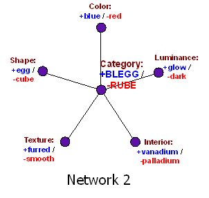
Today, though, I only intend to talk about one particular kind of conditional independence—the case of a central variable that screens off other variables surrounding it, like a central body with tentacles.
Let there be five variables U, V, W, X, Y; and moreover, suppose that for every pair of these variables, one variable is evidence about the other. If you select U and W, for example, then learning U=U1 will tell you something you didn’t know before about the probability W=W1.
An unmanageable inferential mess? Evidence gone wild? Not necessarily.
Maybe U is “Speaks a language”, V is “Two arms and ten digits”, W is “Wears clothes”, X is “Poisonable by hemlock”, and Y is “Red blood”. Now if you encounter a thing-in-the-world, that might be an apple and might be a rock, and you learn that this thing speaks Chinese, you are liable to assess a much higher probability that it wears clothes; and if you learn that the thing is not poisonable by hemlock, you will assess a somewhat lower probability that it has red blood.
Now some of these rules are stronger than others. There is the case of Fred, who is missing a finger due to a volcano accident, and the case of Barney the Baby who doesn’t speak yet, and the case of Irving the IRCBot who emits sentences but has no blood. So if we learn that a certain thing is not wearing clothes, that doesn’t screen off everything that its speech capability can tell us about its blood color. If the thing doesn’t wear clothes but does talk, maybe it’s Nude Nellie.
This makes the case more interesting than, say, five integer variables that are all odd or all even, but otherwise uncorrelated. In that case, knowing any one of the variables would screen off everything that knowing a second variable could tell us about a third variable.
But here, we have dependencies that don’t go away as soon as we learn just one variable, as the case of Nude Nellie shows. So is it an unmanageable inferential inconvenience?
Fear not! for there may be some sixth variable Z, which, if we knew it, really would screen off every pair of variables from each other. There may be some variable Z—even if we have to construct Z rather than observing it directly—such that:
p(u|v,w,x,y,z) = p(u|z)
p(v|u,w,x,y,z) = p(v|z)
p(w|u,v,x,y,z) = p(w|z)
…
Perhaps, given that a thing is “human”, then the probabilities of it speaking, wearing clothes, and having the standard number of fingers, are all independent. Fred may be missing a finger—but he is no more likely to be a nudist than the next person; Nude Nellie never wears clothes, but knowing this doesn’t make it any less likely that she speaks; and Baby Barney doesn’t talk yet, but is not missing any limbs.
This is called the “Naive Bayes” method, because it usually isn’t quite true, but pretending that it’s true can simplify the living daylights out of your calculations. We don’t keep separate track of the influence of clothed-ness on speech capability given finger number. We just use all the information we’ve observed to keep track of the probability that this thingy is a human (or alternatively, something else, like a chimpanzee or robot) and then use our beliefs about the central class to predict anything we haven’t seen yet, like vulnerability to hemlock.
Any observations of U, V, W, X, and Y just act as evidence for the central class variable Z, and then we use the posterior distribution on Z to make any predictions that need making about unobserved variables in U, V, W, X, and Y.
Sound familiar? It should:
As a matter of fact, if you use the right kind of neural network units, this “neural network” ends up exactly, mathematically equivalent to Naive Bayes. The central unit just needs a logistic threshold—an S-curve response—and the weights of the inputs just need to match the logarithms of the likelihood ratios, etcetera. In fact, it’s a good guess that this is one of the reasons why logistic response often works so well in neural networks—it lets the algorithm sneak in a little Bayesian reasoning while the designers aren’t looking.
Just because someone is presenting you with an algorithm that they call a “neural network” with buzzwords like “scruffy” and “emergent” plastered all over it, disclaiming proudly that they have no idea how the learned network works—well, don’t assume that their little AI algorithm really is Beyond the Realms of Logic. For this paradigm of adhockery , if it works, will turn out to have Bayesian structure; it may even be exactly equivalent to an algorithm of the sort called “Bayesian”.
Even if it doesn’t look Bayesian, on the surface.
And then you just know that the Bayesians are going to start explaining exactly how the algorithm works, what underlying assumptions it reflects, which environmental regularities it exploits, where it works and where it fails, and even attaching understandable meanings to the learned network weights.
Disappointing, isn’t it?
- 37 Ways That Words Can Be Wrong by (6 Mar 2008 5:09 UTC; 255 points)
- Dissolving the Question by (8 Mar 2008 3:17 UTC; 163 points)
- Where to Draw the Boundaries? by (13 Apr 2019 21:34 UTC; 125 points)
- Unnatural Categories Are Optimized for Deception by (8 Jan 2021 20:54 UTC; 94 points)
- Information theory and the symmetry of updating beliefs by (20 Mar 2010 0:34 UTC; 65 points)
- Schelling Categories, and Simple Membership Tests by (26 Aug 2019 2:43 UTC; 60 points)
- Timeless Causality by (29 May 2008 6:45 UTC; 50 points)
- Blood Is Thicker Than Water 🐬 by (28 Sep 2021 3:21 UTC; 39 points)
- Blanchard’s Dangerous Idea and the Plight of the Lucid Crossdreamer by (8 Jul 2023 18:03 UTC; 36 points)
- A Hill of Validity in Defense of Meaning by (15 Jul 2023 17:57 UTC; 28 points)
- 's comment on Public beliefs vs. Private beliefs by (5 Jun 2022 13:18 UTC; 17 points)
- Rationality Reading Group: Part N: A Human’s Guide to Words by (18 Nov 2015 23:50 UTC; 9 points)
- 's comment on Blegg Mode by (13 Mar 2019 3:05 UTC; 8 points)
- [SEQ RERUN] Conditional Independence, and Naive Bayes by (15 Feb 2012 5:09 UTC; 7 points)
- 's comment on Blegg Mode by (13 Mar 2019 6:20 UTC; 4 points)
- 's comment on Counterarguments to the basic AI x-risk case by (16 Oct 2022 18:11 UTC; 4 points)
- 's comment on Timeless Causality by (29 May 2008 22:34 UTC; 0 points)
Nice post. However:
Please /please/ don’t use the “+” sign like that! H(X+Y+Z) should be H(X,Y,Z). “So for the joint distribution X+Y there are” should be “So for the joint distribution of X and Y there are” etc. I was skimming your post, misunderstood your meaning entirely and started wondering if you had made a mistake until I went back and noticed that some of your “+”s meant “X and Y” rather than “the value of X plus the value of Y”. (So for example, when I read “”“ Z has two states, “even” and “odd”, perfectly correlated to the evenness or oddness of X+Y. In fact, we’ll suppose that Z is just the question “Are X+Y even or odd?” “”” I thought “golly, ‘Are’ X+Y even or odd? Must be a grammar mistake.”) Now granted, it was easy to tell what you really meant after I slowly read through the introductory paragraph, but please change it, because:
It will confuse mathematicians who are skimming because they’ve seen things like this before
You use the other sense of “+” in your equations, and there’s no excuse for operator overloading if it can be avoided.
The books I’ve read just say “XY” or “X,Y” if they need a name for the joint variable.
It’s not just non-standard, but used inconsistantly. You say H(X+Y+Z) in one place and H(X,Y) in another.
Fair enough—I was just worried that people wouldn’t understand that (X,Y) meant the joint distribution.
Not sure if I’ll get a chance to fix this tonight, I’m at the AGI-08 conference now and may end up in time/sleep deprivation mode.
Fixed.
You forgot to correct an instance of this :
I find it particularly disturbing because in this instance, X+Y is always even...
Two thoughts, which aren’t really coherent or informed enough to be called questions.
If naive Bayes == neural network, and you need 3 layers of neuron to make a general classifier(hyperplanes → convex hulls → arbitrary hypershapes), do you need 3 layers of naive Bayes?
Would an algorithm for inducing names be: poke around looking for things that have mutual information but are not screened off, and induce a name that screens them off. When you find names that have mutual information, decide whether they ought to be merged (a clump of all the pieces has mutual information) or clustered under a hierarchically higher name (otherwise).
My God! For months I thought that your posts had no purpose, but to see it wrapped up like this is beautiful.
This is neat. Two things though:
First a minor mathematical notation quibble/request, specifically about minus signs. Could you move them as much to the outside of a term as possible? What I mean is, for instance, you’ve got the following: H(S) = Sum i: p(Si)*-log2(p(Si))
Personally, I think I’d find H(S) = -Sum i: p(Si)*log2(p(Si)) easier to parse. Probably just due to what I’m used to seeing in mathematical notation, but I seem to see the minus in the middle “before” I see the multiplication, so my initial reaction is “wait, what? subtracting those? huh?” before the rest of my brain catches up and sees it’s actually the expected multiplication by a negated term, just that the negation has been placed in an unusual spot.
Maybe that’s just me though.
Second, just wondering if there’s a simple general principle for knowing when, given a bunch of mutually correlated variables, we can construct a central variable like the above that shields everything from everything else (either completely or at least to a good extent. (Obviously this is tied to how well stuff clusters in conceptspace, but I meant if there’s any relatively simple mathematical criteria)
I’m confused :/
P(X,Y,Z) = P(X,(Y,Z)) = P(X) + P(Y,Z) - P(X;(Y,Z)) = P(X) + (P(Y) + P(Z) - P(Y;Z)) - P(X;(Y,Z)) = P(X) + (P(Y) + P(Z) - P(Y;Z)) - P((X;Y),(X;Z)) = P(X) + (P(Y) + P(Z) - P(Y;Z)) - (P(X;Y) + P(X;Z) - P(X;Y;Z)) = P(X) + P(Y) + P(Z) - P(X;Y) - P(Y;Z) - P(X;Z) + P(X;Y;Z)
By the inclusion-exclusion principle, no?
This was what I expected to see, and I believe it’s equivalent to H(X,Y,Z) = H(X) + H(Y) + H(Z) - I(X;Z) - I(Z;Y) - I(X;Y | Z)
It appears that Z is very artificially constructed—Z is exactly I(X,Y) in the example. Therefore, H(X,Y) = H(X,Y,Z). Since the term I(X,Y | Z) is mutual information about X and Y given Z, that’s just 0. There’s no new mutual information about X and Y that isn’t already in Z. So I believe that we could replace it with +I(X,Y) - I(X,Y,Z), and get inclusion-exclusion.
Hahaha! First thing on LessWrong to really make me laugh out loud :) Good stuff.
[Edit: That’s the laughter of agreement and approval of a fun writing style; I should be more explicit on the internet, given the pernicious amounts of sarcasm that gets tossed around.]
To the downvote, in case it wasn’t clear, I was laughing because I agree with the post, and because “simplify the living daylights out of your calculations” is just an awesome phrase. I laugh at things I agree with way more than things I don’t, because the former things actually make me happy. (And the latter kind of laughter, on the rare occasion that it happens, I keep to myself.)
But if the downvote was for irrelevance, fair enough. I wouldn’t mind being told that expressing appreciation of writing style alone is frowned upon.
It’s a matter of how it’s done. The more analytic and descriptive it is of what was good and how it worked, the better a reaction it’s likely to get.
I would guess that this was downvoted by someone misreading it as an attack, interpreting the laughing as considering it worth ridicule.
It is frowned upon by some people, but not by all—certainly not by me. See discussion here.
Thanks for the background… I think for a compromise, I might just stick to expressing laughter when I happen to have something of content to say along with it :)
A better explanation is probably a parrot.
Possible (?) typo: “V is “Two arms and ten digits”“ could indeed be meant as “V is “Two arms and ten fingers””
Nevermind, didn’t know digits was another word for fingers.