Research Report: Sparse Autoencoders find only 9/​180 board state features in OthelloGPT

[Robert_AIZI]

Link post

[3/​7 Edit: I have rephrased the bolded claims in the abstract per this comment from Joseph Bloom, hopefully improving the heat-to-light ratio.

Commenters have also suggested training on earlier layers and using untied weights, and in my experiments this increases the number of classifiers found, so the headline number should be ³³⁄₁₈₀ features, up from ⁹⁄₁₈₀. See this comment for updated results.]

Abstract

A sparse autoencoder is a neural network architecture that has recently gained popularity as a technique to find interpretable features in language models (Cunningham et al, Anthropic’s Bricken et al). We train a sparse autoencoder on OthelloGPT, a language model trained on transcripts of the board game Othello, which has been shown to contain a linear representation of the board state, findable by supervised probes. The sparse autoencoder finds 9 features which serve as high-accuracy classifiers of the board state, out of 180 findable with supervised probes (and 192 possible piece/​position combinations) [edit: ³³⁄₁₈₀ features, see this comment]. Across random seeds, the autoencoder repeatedly finds “simpler” features concentrated on the center of the board and the corners. This suggests that even if a language model can be interpreted with a human-understandable ontology of interesting, interpretable linear features, a sparse autoencoder might not find a significant number of those features.

Introduction

There has been a recent flurry of research activity around Sparse Autoencoders for Dictionary Learning, a new approach to finding interpretable features in language models and potentially “solving superposition” (Sharkey et al, Anthropic’s Bricken et al, Cunningham et al.). But while this technique can find features which are interpretable, it is not yet clear if sparse autoencoders can find particular features of interest (e.g., features relevant to reducing AI risk).

This research report seeks to answer the question of whether sparse autoencoders can find a set of a-priori existing, interesting, and interpretable features in the OthelloGPT language model. OthelloGPT, as the name suggests, is a language model trained on transcripts of the board game Othello to predict legal moves, but was found to also linearly encode the current board state (Nanda, Hazineh et al). That is, for each of the 64 board positions, there were “board-state features” (linear mappings from the residual stream to \R^3) that classify the state at that position between [is empty] vs [has active-player’s piece] vs [has enemy’s piece], and these board-state features can be found by the supervised training of a linear probe. These board-state features are an exciting testbed for sparse autoencoders because they represent a set of “called-shot” features we hope to find, and which are extremely interpretable and correspond to natural human thinking^[1]. If the sparse autoencoder can find these features, this is some evidence that they will find relevant and important features in language models. Conversely, if the sparse autoencoders can’t find these features, that indicates a limitation of the method, and provides a test case where we can adjust our training methods until we can find them.

Overview

Here we:

1. Train an OthelloGPT model from scratch

2. Train a linear probe to classify the board states (replicating Hazineh et al) from an intermediate layer of OthelloGPT.

3. Train a sparse autoencoder on the same layer of OthelloGPT

4. Assess whether the features found by the sparse autoencoder include the linear encoding of the current board state that the linear probe is able to find.

5. Retrain the sparse autoencoder with different random seeds, and analyze which features are found.

An overview of the approach

Methods

Training OthelloGPT

We first trained an OthelloGPT model from scratch, following the approach of Li et al. Our model is a 25M parameter, 8-layer, decoder-only transformer, with residual stream dimension d_model=512 (identical to Li et al’s model). It is trained to do next-token-prediction of random transcripts of Othello games, with each possible move being encoded as a separate token, resulting in a vocabulary size of 66 (64 from the positions on the boards, plus 2 special tokens). The model was trained on a corpus of 640K games for 2 epochs, using the Adam optimizer with learning rate 1e-3.

The trained model had a 5% error rate in predicting next legal moves. This is far higher than Li et al’s 0.01%, which I believe is due to my shorter training run on smaller data^[2]. Despite this relatively high error rate, the model has been trained to a point where it exhibits the linearly-encoded board state described by Hazineh et al, which we will show in the next section.

Training Linear Probes

We next train linear probes using its residual stream to classify the contents of individual board positions. This serves two purposes: first to confirm that our OthelloGPT model linearly encodes the board state, and secondly serves as a baseline for the classification accuracy we can expect from any sparse autoencoder features.

As in Nanda and Hazineh et al, we found that we could train higher accuracy probes if we group positions into “empty/​own/​enemy” rather than “empty/​black/​white”. Following Nanda’s recommendation, we trained our probes on the residual stream of the model just after the MLP sublayer of layer 6. Each probe is a linear classifier from the residual stream (\R^512) to the three classes (\R^3), trained to minimize cross-entropy between the true labels of the board state, and the classifier’s predictions. We train one probe for each of the 64 board positions, resulting in 3*64 directions in activation space^[3]. As in Nanda’s work, we found that our classifiers had a greater accuracy if we restricted them to the “middle” turns of each Othello game, in our case turns [4, 56). The probes were trained on 100K labelled games, for 1 epoch, using the Adam optimizer with learning rate 1e-3.

The resulting probes predict board positions with an error rate of 10%. While this is much larger than Hazineh et al’s 0.5% error rate, it is far better than chance, and indicates that there is linear structure to find. We also measure classification accuracy with AUROC, since this allows us to compare probe and feature directions as classifiers. In particular, for each position, for classes A/​B/​C with scores a/​b/​c, we use the “rectified directions” a-0.5(b+c) as a score for class A vs (B or C). We find that all of the 192 rectified probe directions have an AUROC greater than .9, with the exception of the 12 features corresponding to the central 4 tiles (which begin the game filled, and therefore might be handled differently by the language model). We will therefore use .9 as the (semi-arbitrary) threshold for a “high accuracy” classifier.

A histogram of the AUROC classification accuracies of the 192 probe directions. Almost all probe directions serve as a classifier with AUROC at least .9. The small bar at 0.5 is an artifact of measuring AUROC when there is only one class, corresponding to the 4 central tiles being classified as empty/​(own+enemy). The other bar below .9 corresponds to the 8 probes for classifying those central tiles as own/​(empty+enemy) or enemy/​(own+empty).

A density plot of the rectified probe activations for position 26 across the test set. The rectified probe scores cleanly classify Empty positions, and make some progress at classifying Enemy and Own positions.

Training The Sparse Autoencoder

Our sparse autoencoder architecture is based on that in Cunningham et al, consisting of a single hidden layer with ReLU activations, tied encoder-decoder weights and a bias on the encoder but not decoder layer. As with the probes, we trained on layer 6 of the GPT model, and turns [4, 56). We used a feature ratio R=2 (1024 features for a 512-dimensional model), and a sparsity coefficient α=7.7e-2. This sparsity coefficient was chosen after a hyperparameter sweep in order to minimize the sum of unexplained variance and average number of features active. The autoencoder was trained on a corpus of 100K games for 4 epochs, using the Adam optimizer with learning rate 1e-3.

The resulting autoencoder had an average of 12% features active, 17% unexplained variance, and 0.2% dead features on the test set.

Results

SAE Features as Current-Board Classifiers

For each of the 1024 sparse autoencoder features, we can measure if they correctly classify the current board state as an empty/​own/​enemy piece. We find that there are several features which serve as highly accurate classifiers for whether a tile is empty.

Feature 395 has a high activation when Position 43 is empty, and activates less (or not at all) when there is a piece there. Data is from a test set of 2000 games. Feature scores of 0 have been separated out into the bar on the left. Depicted AUROC is .9999.

Visual inspection of the boards confirms that Feature 395 correctly classifies if position 43 is empty or filled:

(Top) The five Othello boards that most activated Feature 395. (Bottom) Five random boards. Feature activations are shown, and the feature with a cutoff of 30 correctly predicts if Position 43 (D6, marked with a red circle) is filled.

The sparse autoencoder found 9 features which act as classifiers with AUROC>.9, all for assessing when the tile is empty vs (own+enemy). The best non-empty classifier is Feature 525, classifying Position 7 with an AUROC of .86:

Feature 525 activates more when position 7 has an enemy piece, and less when it is empty or has your own piece. AUROC shown is .86.

Here are the top- and random-activating examples for this feature:

(Top) The five Othello boards that most activated Feature 525. (Bottom) Five random boards. Feature activations are shown, and the feature often, though not always, predicts if Position 7 (H1, marked with a red circle) has an enemy piece (denoted as white).

It should be noted that both of these classification tasks are computationally simpler that the other classification tasks: checking if a tile is empty is just querying the context window for the corresponding token, and since corners cannot be flipped, checking if a corner is an enemy piece is just querying the context window for that token an odd number of turns ago. (Though that’s not what the classifiers are doing, at least directly, since they only have access to the residual stream and not the tokens themselves.)

The feature best at classifying a non-corner, non-empty token is feature 688, which has an AUROC of .828:

Feature 688 activates more when position 15 has a piece than when it is empty, but just barely differentiates enemy pieces from its own pieces. AUROC shown is 0.828.

Overall, the sparse autoencoder has found some classifier features, but the vast majority of features do not classify the current board state, and the majority of board states are not well-classified by features. The features that are good classifiers correspond to “easier” classification tasks, ones that do not engage with the complexities of pieces flipping.

Which Features are Learned?

Knowing that only some classifiers are found by the sparse autoencoder, we should ask:

1. Which classifiers?

2. Are these directions “easier to find”, or would the autoencoder find other ones if retrained?

To test this, I trained the autoencoder 10 times, with different random seeds, and investigated which features were found. The only differences between these autoencoder training runs were: the initialization of the autoencoder weights, and the ordering of the training data (though the overall training set was the same).

I then checked if each autoencoder had a feature which acts as a classifier for a position with AUROC>.9. This is the result:

The sparse autoencoder is likely to find features which classify the inner ring of tiles, and the corners. Sparse autoencoders almost never find good classifiers for other positions. Except for the corner tiles, all classifiers with AUROC>.9 were for whether the position was empty vs filled.

This indicates that the inner-ring features are in some way easier for the autoencoder to learn, either due to the dataset used or the way OthelloGPT represents them. It seems likely that these are the most prominent features to learn since these moves are playable from the beginning of the game, and that these moves have important effects on whether other moves are playable. The lack of classifiers for the central tiles is explained by the difficulty of classifying these tiles even with linear probes (recall that the probes there had AUROC<.9). The corner classifiers also seem to be easier to learn, and are the only features with AUROC>.9 which classify enemy vs own pieces.

Overall, we can conclude that the autoencoder has a preference for learning some features over others. These features might be more “prominent” in the residual stream, or in the dataset, or in some other way, and I have not tested these hypotheses yet.

SAE Features as Legal-Move Classifiers

Since the model is trained to predict legal moves, one might expect it to learn features for if a move is legal. And unlike in the autoencoders-on-text case, there are fewer tokens than autoencoder features, so it would be easy to allocate 60/​1024 features for predicting tokens, if that is useful to the sparse autoencoder.

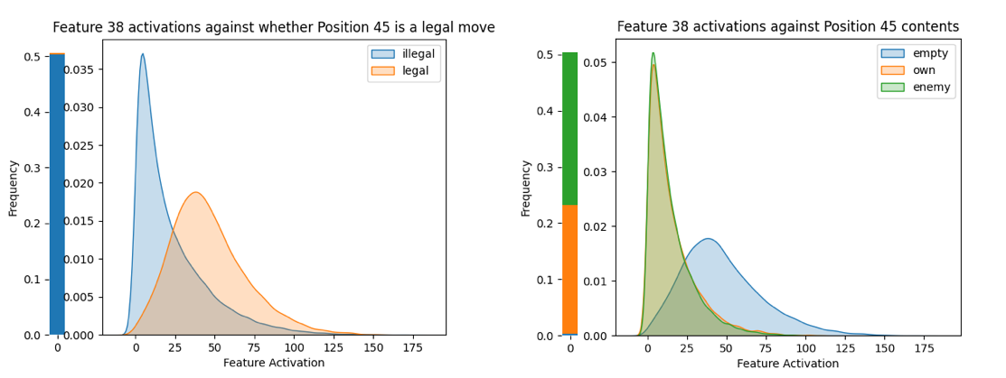
We find the autoencoder often finds features that classify whether a move is legal. However, this is confounded by the overlap of “move is legal” and “tile is empty” (the former is the later plus some extra conditions). There were several features that are decent legal-move classifiers, but when you look at their activation distributions its clear they are actually empty-tile classifiers that score well on legal move classification because P(legal | empty) was high:

Feature 722 has a high AUROC as a legal-move classifier for position 26, but is an even better classifier of whether position 26 is empty. Its high accuracy at classifying legal moves can be explained by classifying if the square is empty, plus applying the incorrect logic “empty → legal”.

Some density plots looked like Feature 722/​Position 26, showing clear confounding, and other look like this, where the distributions are nearly identical:

Finally, we can compare the AUROCs of the probes to the SAE features (both as content predictors and legal move predictors):

Histogram of AUROCs for: (Left) probe directions doing content prediction (identical to a previous figure). (Center) For each position/​content pair, the best AUROC of a sparse autoencoder feature at classifying that pair. (Right) For each position/​legality pair, the best AUROC of a sparse autoencoder feature at classifying that pair. The probe directions are concentrated near AUROC=1, while both assessments of the SAE features are more levelly distributed around AUROC=.7, with a tail to the right and a small spike near AUROC=1.

Cosine Similarities

Finally, we can directly compare the directions found by probes and the autoencoders. In particular, for each of the 192 rectified probe directions, we computed its maximum cosine similarity across the 1024 autoencoder directions. This is the result:

(Blue, left axis) Histogram of maximum cosine similarities of probe directions with autoencoder directions. (Orange, right axis) Maximum cosine similarities of probe directions with random vectors, acting as a control group. The probe directions have much higher MCS than would be expected from chance, but never exceed a cosine similarity of .7.

We can conclude that the autoencoder directions are relatively close to the probe directions in activation space, but do not perfectly match. We shouldn’t be worried about this lack of perfect matching since a correlation of .6 is enough both in theory and in practice for the autoencoder features to be ~perfect classifiers.

One Really Cool Case Study

As I was investigating high-correlation features that were bad classifiers (by AUROC), I found several features like this one, which shows clear bimodality that isn’t aligned with empty/​own/​enemy pieces:

Feature 348’s activations are bimodal, with a large peak near 0 and a smaller peak near 50. The peak near 0 is a mixture of empty/​own/​enemy pieces, but the peak at 50 is only for enemy pieces.

For this feature, when I looked at the top-activating boards, I found them to be highly interpretable. See if you can spot the pattern:

Top and random activating boards for feature 348.

It looks like this feature activates when positions F2-F6 are all white! And what’s incredible is the “partial activation” in the bottom row: the feature activates at 12 when positions E2-E6 are all white! That seems like an extremely understandable “near-miss” for the feature, which is astonishing to me.

We should here acknowledge that Othello and OthelloGPT can be harder to interpret than English text. Whereas humans will find patterns and themes in text for fun, I found my brain was very much not wired for analyzing Othello boards, and therefore in most cases I could only test feature interpretability by programmatically testing individual hypotheses. Therefore, I have not been able to analyze the vast majority of OthelloGPT features, and they may have interpretable meanings like the above that simply do not show up on my metrics. If anyone wants to do a lot of case studies of individual features, I’m happy to share the tools I have.

Conclusion

We have shown that out of a set of 180 a-priori interesting and interpretable features in OthelloGPT, sparse autoencoders find only 9 of them. While this confirms the promise of sparse autoencoders in Cunningham et al and Bricken et al, that they find interpretable features, it also underlines the limitations of the approach: this is the first work demonstrating that sparse autoencoders can fail to find a concrete set of interesting, interpretable features, and suggests that currently-existing sparse autoencoders cannot “fully” interpret a language model. We hope that these results will inspire more work to improve the architecture or training methods of sparse autoencoders to address this shortcoming. Finally, we hope we have shown that OthelloGPT, with its linear world state, is useful for measuring if unsupervised techniques find important interpretable directions, and can be a fruitful place to test interpretability techniques.

Future work:

1. Redo this analysis on the fully-trained OthelloGPT created by Li et al.

2. Adjust the autoencoder architecture until it is able to find more of the features we hope to see. Possible architectural changes include:

   1. Untied encoder/​decoder weights as in Anthropic’s Bricken et al.

   2. Update the architecture using the tricks described in Anthropic’s updates.

   3. Update the loss function to include an orthogonality penalization term, as described by Till.

3. (Low-priority) Redo this analysis on the MLP layer of the transformer (as Bricken et al do) instead of the residual stream. (The MLP layers may not linearly represent the board state, so first we’d want to verify this with a new set of probes.)

4. (Low-priority) Continue investigating individual autoencoder features.

1. ^

   Though, notably, this was not the first way people expected OthelloGPT to encode the board state. Since humans conceptualize Othello as a game between two players, the original authors tried to find linear features representing whether a square was empty/​black/​white. The resulting classifiers were mediocre, with an error rate of 20% or more. However, Neel Nanda found that since the language model “plays both sides”, it linearly encodes the board as empty/​own/​enemy pieces (i.e., grouping “black on even turns” with “white on odd turns” instead of “black on odd turns”), and Hazineh et al find probes trained to do this classification can have an error rate as low as 0.5%.

2. ^

   I plotted OthelloGPT’s error rate across its training, and it followed a straightforward scaling law that would have reached 0.01% error rate with a few more OOMs of training data. I opted not to train to that level, but I plan to redo my analyses on Li et al’s OthelloGPT when I can get my hands on it.

3. ^

   Though we should note that the relative difference between two directions is more important the directions themselves. Since the predictions go through a softmax, the classifier with directions (A,B,C) produces the same results as with directions (A+X, B+X, C+X) for any X. The invariant properties learned by the classifier are the differences B-A and C-A, or the “rectified directions” like A-0.5(B+C).

[Joseph Bloom]

Thanks for posting this! I’ve had a lot of conversations with people lately about OthelloGPT and I think it’s been useful for creating consensus about what we expect sparse autoencoders to recover in language models.

Maybe I missed it but:

• What is the performance of the model when the SAE output is used in place of the activations?

• What is the L0? You say 12% of features active so I assume that means 122 features are active.This seems plausibly like it could be too dense (though it’s hard to say, I don’t have strong intuitions here). It would be preferable to have a sweep where you have varying L0′s, but similar explained variance. The sparsity is important since that’s where the interpretability is coming from. One thing worth plotting might be the feature activation density of your SAE features as compares to the feature activation density of the probes (on a feature density histogram). I predict you will have features that are too sparse to match your probe directions 1:1 (apologies if you address this and I missed this).

• In particular, can you point to predictions (maybe in the early game) where your model is effectively perfect and where it is also perfect with the SAE output in place of the activations at some layer? I think this is important to quantify as I don’t think we have a good understanding of the relationship between explained variance of the SAE and model performance and so it’s not clear what counts as a “good enough” SAE.

I think a number of people expected SAEs trained on OthelloGPT to recover directions which aligned with the mine/​their probe directions, though my personal opinion was that besides “this square is a legal move”, it isn’t clear that we should expect features to act as classifiers over the board state in the same way that probes do.

This reflects several intuitions:

1. At a high level, you don’t get to pick the ontology. SAEs are exciting because they are unsupervised and can show us results we didn’t expect. On simple toy models, they do recover true features, and with those maybe we know the “true ontology” on some level. I think it’s a stretch to extend the same reasoning to OthelloGPT just because information salient to us is linearly probe-able.

2. Just because information is linearly probeable, doesn’t mean it should be recovered by sparse autoencoders. To expect this, we’d have to have stronger priors over the underlying algorithm used by OthelloGPT. Sure, it must us representations which enable it to make predictions up to the quality it predicts, but there’s likely a large space of concepts it could represent. For example, information could be represented by the model in a local or semi-local code or deep in superposition. Since the SAE is trying to detect representations in the model, our beliefs about the underlying algorithm should inform our expectations of what it should recover, and since we don’t have a good description of the circuits in OthelloGPT, we should be more uncertain about what the SAE should find.

3. Separately, it’s clear that sparse autoencoders should be biased toward local codes over semi-local /​ compositional codes due to the L1 sparsity penalty on activations. This means that even if we were sure that the model represented information in a particular way, it seems likely the SAE would create representations for variables like (A and B) and (A and B’) in place of A even if the model represents A. However, the exciting thing about this intuition is it makes a very testable prediction about combinations of features likely combining to be effective classifiers over the board state. I’d be very excited to see an attempt to train neuron-in-a-haystack style sparse probes over SAE features in OthelloGPT for this reason.

Some other feedback:

• Positive: I think this post was really well written and while I haven’t read it in more detail, I’m a huge fan of how much detail you provided and think this is great.

• Positive: I think this is a great candidate for study and I’m very interested in getting “gold-standard” results on SAEs for OthelloGPT. When Andy and I trained them, we found they could train in about 10 minutes making them a plausible candidate for regular /​ consistent methods benchmarking. Fast iteration is valuable.

• Negative: I found your bolded claims in the introduction jarring. In particular “This demonstrates that current techniques for sparse autoencoders may fail to find a large majority of the interesting, interpretable features in a language model”. I think this is overclaiming in the sense that OthelloGPT is not toy-enough, nor do we understand it well enough to know that SAEs have failed here, so much as they aren’t recovering what you expect. Moreover, I think it would best to hold-off on proposing solutions here (in the sense that trying to map directly from your results to the viability of the technique encourages us to think about arguments for /​ against SAEs rather than asking, what do SAEs actually recover, how do neural networks actually work and what’s the relationship between the two).

• Negative: I’m quite concerned that tieing the encoder /​ decoder weights and not having a decoder output bias results in worse SAEs. I’ve found the decoder bias initialization to have a big effect on performance (sometimes) and so by extension whether or not it’s there seems likely to matter. Would be interested to see you follow up on this.

Oh, and maybe you saw this already but an academic group put out this related work: https://​​arxiv.org/​​abs/​​2402.12201 I don’t think they quantify the proportion of probe directions they recover, but they do indicate recovery of all types of features that been previously probed for. Likely worth a read if you haven’t seen it.

[Robert_AIZI]

I’ve had a lot of conversations with people lately about OthelloGPT and I think it’s been useful for creating consensus about what we expect sparse autoencoders to recover in language models.

I’m surprised how many people have turned up trying to do something like this!

What is the performance of the model when the SAE output is used in place of the activations?

I didn’t test this.

What is the L0? You say 12% of features active so I assume that means 122 features are active.

That’s correct. I was satisfied with 122 because if the SAEs “worked perfectly” (and in the assumed ontology etc) they’d decompose the activations into 64 features for [position X is empty/​own/​enemy], plus presumably other features. So that level of density was acceptable to me because it would allow the desired ontology to emerge. Worth trying other densities though!

In particular, can you point to predictions (maybe in the early game) where your model is effectively perfect and where it is also perfect with the SAE output in place of the activations at some layer? I think this is important to quantify as I don’t think we have a good understanding of the relationship between explained variance of the SAE and model performance and so it’s not clear what counts as a “good enough” SAE.

I did not test this either.

At a high level, you don’t get to pick the ontology.

I agree, but that’s part of what’s interesting to me here—what if OthelloGPT has a copy of a human-understandable ontology, and also an alien ontology, and sparse autoencoders find a lot of features in OthelloGPT that are interpretable but miss the human-understandable ontology? Now what if all of that happens in an AGI we’re trying to interpret? I’m trying to prove by example that “human-understandable ontology exists” and “SAEs find interpretable features” fail to imply “SAEs find the human-understandable ontology”. (But if I’m wrong and there’s a magic ingredient to make the SAE find the human-understandable ontology, lets find it and use it going forward!)

Separately, it’s clear that sparse autoencoders should be biased toward local codes over semi-local /​ compositional codes due to the L1 sparsity penalty on activations. This means that even if we were sure that the model represented information in a particular way, it seems likely the SAE would create representations for variables like (A and B) and (A and B’) in place of A even if the model represents A. However, the exciting thing about this intuition is it makes a very testable prediction about combinations of features likely combining to be effective classifiers over the board state. I’d be very excited to see an attempt to train neuron-in-a-haystack style sparse probes over SAE features in OthelloGPT for this reason.

I think that’s a plausible failure mode, and someone should definitely test for it!

I found your bolded claims in the introduction jarring. In particular “This demonstrates that current techniques for sparse autoencoders may fail to find a large majority of the interesting, interpretable features in a language model”.

I think our readings of that sentence are slightly different, where I wrote it with more emphasis on “may” than you took it. I really only mean this as an n=1 demonstration. But at the same time, if it turns out you need to untie your weights, or investigate one layer in particular, or some other small-but-important detail, that’s important to know about!

Moreover, I think it would best to hold-off on proposing solutions here

I believe I do? The only call I intended to make was “We hope that these results will inspire more work to improve the architecture or training methods of sparse autoencoders to address this shortcoming.” Personally I feel like SAEs have a ton of promise, but also could benefit from a battery of experimentation to figure out exactly what works best. I hope no one will read this post as saying “we need to throw out SAEs and start over”.

Negative: I’m quite concerned that tieing the encoder /​ decoder weights and not having a decoder output bias results in worse SAEs.

That’s plausible. I’ll launch a training run of an untied SAE and hopefully will have results back later today!

Oh, and maybe you saw this already but an academic group put out this related work: https://​​arxiv.org/​​abs/​​2402.12201

I haven’t seen this before! I’ll check it out!

[Robert_AIZI]

Followup on tied vs untied weights: it looks like untied makes a small improvement over tied, primarily in layers 2-4 which already have the most classifiers. Still missing the middle ring features though.

Next steps are using the Li et al model and training the SAE on more data.

[Charlie Steiner]

At a high level, you don’t get to pick the ontology.

This post seems like a case of there being too many natural abstractions.

[vlad k]

Thank you for sharing! I am also working on a write-up post for experiments I conducted with SAEs trained on Othello-GPT:) I’m using the original model by Kenneth Li et al., and mostly training SAEs with 512-1024 features. I also found that simple features such as my/​their/​empty are indeed rarely found in SAEs trained on later layers. However, there are more of them in SAEs trained on middle layers (including cells outside the “inner-ring”). In later layers, SAEs usually learn more complicated features, such as the combination of a few close cells being of a particular type. It makes sense because, by the last layer, all you care about are the complex features “is this move valid”, and simple features gradually become less relevant (and will probably have lesser norm). I’m hoping to share some more of my findings soon.

[Robert_AIZI]

[Continuing our conversation from messages]

I just finished a training run of SAEs on the intermediate layer of my OthelloGPT. For me it seemed like the sweet spot was layers 2-3, and the SAE found up to 30 high-accuracy classifiers on Layer 3. They were located all in the “inner ring” and “outer ring”, with only one in the “middle ring”. (As before, I’m counting “high-accuracy” as AUROC>.9, which is an imperfect metric and threshold.)

Here were the full results. The numbers/​colors indicate how many classes had a high-accuracy classifier for that position.

[Zechen Zhang]

This is an interesting point—when we did our causality studies across layers, we also found that the board state features in the middle layers are mostly used causally—not the deep layers. However, the probe accuracy does increase with depth.

I don’t know how this translates to the fact that SAEs also find more of these features in the middle layers. Like, the “natural features” in some sense in the last few layers found by the SAEs do not have to contain much information about the board state but just partial information to make the decision.

[LawrenceC]

Thanks for doing this—could you share your code?

While I put only a medium probability that the current SAE algorithm works to recover all the features, my main concerns with the work are due to the quality of the model and the natural “features” not being board positions.

I’d be interested in running the code on the model used by Li et al, which he’s hosted on Google drive:

https://​​drive.google.com/​​drive/​​folders/​​1bpnwJnccpr9W-N_hzXSm59hT7Lij4HxZ

Also, in addition to the future work you list, I’d be interested in running the SAEs with much larger Rs and with alternative hyperparameter selection criteria.

[Robert_AIZI]

Thanks for doing this—could you share your code?

Just uploaded the code here: https://​​github.com/​​RobertHuben/​​othellogpt_sparse_autoencoders/​​. Apologies in advance, the code is kinda a mess since I’ve been writing for myself. I’ll take the hour or so to add info to the readme about the files and how to replicate my experiments.

I’d be interested in running the code on the model used by Li et al, which he’s hosted on Google drive:

https://​​drive.google.com/​​drive/​​folders/​​1bpnwJnccpr9W-N_hzXSm59hT7Lij4HxZ

Thanks for the link! I think replicating the experiment with Li et al’s model is definite next step! Perhaps we can have a friendly competition to see who writes it up first :)

I have mixed feelings about whether the results will be different with the high-accuracy model from Li et al:

1. On priors, if the features are more “unambiguous”, they should be easier for the sparse autoencoder to find.

2. But my hacky model was at least trained enough that those features do emerge from linear probes. If sparse autoencoders can’t match linear probes, thats also worth knowing.

3. If there is a difference, and sparse autoencoders work on a language model that’s sufficiently trained, would LLMs meet that criteria?

Also, in addition to the future work you list, I’d be interested in running the SAEs with much larger Rs and with alternative hyperparameter selection criteria.

Agree that its worth experimenting with R, but the only other hyperparameter is the sparsity coefficient alpha, and I found that alpha had to be in a narrow range or the training would collapse to “all variance is unexplained” or “no active features”. (Maybe you mean Adam hyperparameters, which I suppose might also be worth experimenting with.) Here’s the result of my hyperparameter sweep for alpha:

[leogao]

Fwiw, I find it’s much more useful to have (log) active features on the x axis, and (log) unexplained variance on the y axis. (if you want you can then also plot the L1 coefficient above the points, but that seems less important)

[Robert_AIZI]

Good thinking, here’s that graph! I also annotated it to show where the alpha value I ended up using for the experiment. Its improved over the pareto frontier shown on the graph, and I believe thats because the data in this sweep was from training for 1 epoch, and the real run I used for the SAE was 4 epochs.

[leogao]

In my experiments log L0 vs log unexplained variance should be a nice straight line. I think your autoencoders might be substantially undertrained (especially given that training longer moves off the frontier a lot). Scaling up the data by 10x or 100x wouldn’t be crazy.

(Also, I think L0 is more meaningful than L0 /​ d_hidden for comparing across different d_hidden (I assume that’s what “percent active features” is))

[LawrenceC]

Thanks for uploading your interp and training code!

Could you upload your model and/​or datasets somewhere as well, for reproducibility? (i.e. your datasets folder containing the datasets:)

def recognized_dataset():
    mode_lookups={
        "gpt_train":        ["datasets/othello_gpt_training_corpus.txt",        OthelloDataset,         {}],
        "gpt_train_small":  ["datasets/small_othello_gpt_training_corpus.txt",  OthelloDataset,         {}],
        "gpt_test":         ["datasets/othello_gpt_test_corpus.txt",            OthelloDataset,         {}],
        "sae_train":        ["datasets/sae_training_corpus.txt",                OthelloDataset,         {}],
        "probe_train":      ["datasets/probe_train_corpus.txt",                 LabelledOthelloDataset, {}],
        "probe_train_bw":   ["datasets/probe_train_corpus.txt",                 LabelledOthelloDataset, {"use_ally_enemy":False}],
        "probe_train_small":["datasets/small_probe_training_corpus.txt",        LabelledOthelloDataset, {}],
        "probe_test":       ["datasets/probe_test_corpus.txt",                  LabelledOthelloDataset, {}],
    }
    return mode_lookups

Agree that its worth experimenting with R, but the only other hyperparameter is the sparsity coefficient alpha, and I found that alpha had to be in a narrow range or the training would collapse to “all variance is unexplained” or “no active features”.

Yeah, the main hyperparameters are the expansion factor and “what optimization algorithm do you use/​what hyperparameters do you use for the optimization algorithm”.

[Robert_AIZI]

Here are the datasets, OthelloGPT model (“trained_model_full.pkl”), autoencoders (saes/​), probes, and a lot of the cached results (it takes a while to compute AUROC for all position/​feature pairs, so I found it easier to save those): https://​​drive.google.com/​​drive/​​folders/​​1CSzsq_mlNqRwwXNN50UOcK8sfbpU74MV

You should download all of these into the same level directory as the main repo.

[Joseph Bloom]

@LawrenceC Nanda MATS stream played around with this as group project with code here: https://​​github.com/​​andyrdt/​​mats_sae_training/​​tree/​​othellogpt

[Robert_AIZI]

Cool! Do you know if they’ve written up results anywhere?

[Joseph Bloom]

I think we got similar-ish results. @Andy Arditi was going to comment here to share them shortly.

[Andy Arditi]

We haven’t written up our results yet.. but after seeing this post I don’t think we have to :P.

We trained SAEs (with various expansion factors and L1 penalties) on the original Li et al model at layer 6, and found extremely similar results as presented in this analysis.

It’s very nice to see independent efforts converge to the same findings!

[Robert_AIZI]

Likewise, I’m glad to hear there was some confirmation from your team!

An option for you if you don’t want to do a full writeup is to make a “diff” or comparison post, just listing where your methods and results were different (or the same). I think there’s demnad for that, people liked Comparing Anthropic’s Dictionary Learning to Ours

[LawrenceC]

Thanks!

[Charlie Steiner]

Had a chat with @Logan Riggs about this. My main takeaway was that if SAEs aren’t learning the features for separate squares, it’s plausibly because in the data distribution there’s some even-more-sparse pattern going on that they can exploit. E.g. if big runs of same-color stones show up regularly, it might be lower-loss to represent runs directly than to represent them as made up of separate squares.

If this is the bulk of the story, then messing around with training might not change much (but training on different data might change a lot).

[Charlie Steiner]

Nice! This was a very useful question to ask.

[Caridorc Tergilti]

Did you use ghost gradients? (gradients that tend to reactivate features that are at zero)

[Robert_AIZI]

Nope. I think they wouldn’t make much difference—at the sparsity loss coefficient I was using, I had ~0% dead neurons (and iirc the ghost gradients only kick in if you’ve been dead for a while). However, it is on the list of things to try to see if it changes the results.