[Research Update] Sparse Autoencoder features are bimodal

Overview

The sparse autoencoders project is a mechanistic interpretability effort to algorithmically find semantically meaningful “features” in a language model. A recent update hints that features learned by this approach separate into two types depending on their maximum cosine similarity (MCS) score against a larger feature dictionary:

High-MCS features that reoccur across hyperparameters (speculatively, the “real” features that would be helpful for mechanistic interpretability)
Low-MCS features that do not reoccur (speculatively, dead neurons or artifacts of random noise)

Figure 1: Figure 3 from the replication, showing that MCS scores are bimodal, with peaks near MCS=.3 and MCS=1.

In this post, we:

Demonstrate that the MCS distribution of the low-MCS features matches the distribution of random vectors.
Present data show that a feature’s MCS against two larger models are highly correlated.
Show that as the size of the feature dictionary increases, the number of features which are high-MCS increases, even as their proportion decreases.

Thanks to Hoagy Cunningham for providing the model weights, answering my questions, and feedback on this draft, and to Dan Braun, Beren Millidge, Logan Riggs, and Lee Sharkey for producing the work that motivates this post.

Background

[Feel free to skip or skim this section if you’re already familiar with the project. Original sources: the Interim Research Report, my summary, the replication.]

Our goal is to extract features from the internal activations of a transformer language model. We used this small language model, as described in the replication:

We used Andrej Karpathy’s nanoGPT to train a small transformer, with 6 layers, a 32 dimensional residual stream, MLP widths of 128 and 4 attention heads with dimension 8. We trained on a node of 4xRTX3090s for about 9h, reaching a loss of 5.13 on OpenWebText.

The internal activations of this model’s MLP in layer 2 (d=128) are used to train an autoencoder as described in my summary. In fact, six autoencoders are trained, each with L^1 penalty coefficient α=0.001, but with different “dictionary size” J, ranging across the set {256, 512, 1024, 2048, 4096, 8192}, and different random initializations.

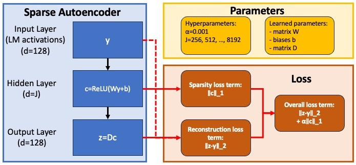
Figure 2: An overview of the sparse autoencoder architecture, the loss function used in its training, and its (hyper)parameters.

The product of interest from this training process is the resulting feature dictionary D, a 128-by-J matrix, which we interpret as J vectors in 128-dimensional activation space, the “features” of the language model^[1].

Given a feature and a dictionary D, we use the metric of maximum cosine similarity (MCS) to measure the extent to which this feature is found by the dictionary. MCS is, as the name suggests, the greatest cosine similarity between that feature and a feature in the dictionary D. MCS takes values in the range [-1,1], with larger values meaning the feature is closer to being in the dictionary (and 1 meaning the feature is exactly in the dictionary). More often, we will compute MCS between two dictionaries, resulting in a distribution of MCS scores for each feature in the first dictionary, scored against the second dictionary.

The Low-MCS distribution matches a random MCS distribution

In the replication it was noted that this distribution of MCS scores is bimodal, consisting of a peak near MCS=1, and a peak near MCS=0.3.

Figure 3: Distribution of maximum cosine similarities from the 1024-feature dictionary, measured against the 8192-feature dictionary. Note the two peaks, near MCS=.3 and MCS=1.

In this section, we will consider just the part of the distribution where MCS<.5, and demonstrate that its nearly identical to a distribution generated at random from computing MCS between two dictionaries.

To generate the distributions, we compute MCS between two dictionaries, then throw out all data above a cutoff of MCS=.5. For the “learned” dataset, we use the two dictionaries produced by training runs of the autoencoders. For the “random” dataset, we use dictionaries generated by sampling each entry are sampled from the standard normal distribution N(0,1)^[2].

The resulting frequency histograms look remarkably similar:

Figure 4: Comparison of MCS<.5 frequencies between learned and random dictionaries, which are remarkably similar. The blue bars are the same data as in the previous diagram.

This similarity is consistent as you vary the size of the learned dictionary^[3]:

Figure 5: Comparison of MCS<.5 frequencies between learned and random dictionaries, of varying sizes.

To quantify the degree of similarity between these distributions, we use the Wasserstein metric, also called earthmover distance (EMD)^[4]. Intuitively, EMD is the minimal amount of mass*distance you’d have to move to rearrange one distribution to another. Since EMD is a metric, smaller values mean closer, with 0 EMD meaning identical distributions.

In order to provide context for the EMD values, I generated multiple random-feature MCS distributions, and computed EMD between all of them, as well as the original data. Here is the resulting distance chart for dictionaries of size 1024 and 8192:

Figure 6: Earthmover distances between the learned features and four sets of random features (in all cases, 1024-feature dictionaries being compared to 8192-feature dictionaries). On the whole, the random MCS datasets are closer to each other than to the MCS set from the learned dictionary, but the values are within a factor of 2. There’s one instance where the learned dataset is closer to a random dataset than a random dataset is to another random dataset: EMD(learned, rand2)<EMD(rand1,rand2).

As another benchmark, we can compare against a random MCS set generated by different parameters. In this case, Rand 1-Rand 4 are generated with 1024 features taking maximum cosine similarity against a dictionary of M=8192 features, while the “Alt param” distribution takes the MCS of 1024 features against a dictionary of M=2*8192 features.

Figure 7: As the previous diagram, with one additional distribution, “Alt Params”, generated as a random distribution between 1024 vs 16384 features, instead of the 1024 vs 8192 features for other distributions. Note that the learned distribution and the random distributions are all much closer to each other than to the Alt Params distribution.

These trends are similar across feature dictionaries of size 1024, 2048, and 4096 (but to a lesser extent for size 512):

Figure 8: Four versions of the previous diagram for feature dictionaries of varying sizes.

Overall, we believe this data suggests that the MCS scores of low-MCS features are well-explained by being unrelated to the larger feature dictionary. There could be several reasons such features being unrelated:

The low-MCS features are dead neurons.
The low-MCS features are trying to account for “noise” in the transformer or in the selection of training vectors.
The low-MCS features are semantically meaningful, but were simply not found by the larger feature dictionary.

We do not yet have evidence for one of these explanations over another, nor have we ruled out other explanations.

Features’ MCS scores against larger dictionaries are highly correlated

Taking a small dictionary and two larger dictionaries, we can compute the MCS of a feature in the small dictionary against one larger dictionary, then the other. This results in two MCS scores, which are highly correlated, due to large clusters near (.3, .3) and (1,1):

Feature 9: Scatter plot where each point represents a feature in the size-1024 dictionary. Its x value is the MCS of that feature against the size 2048 dictionary, and its y-value is its MCS against the size 4096 dictionary. Note the large clusters near (.3,.3) and (1,1).

We get similar results comparing other sizes of dictionaries:

Feature 10: As previous diagram but for a smaller feature dictionary.

Finding more features finds more high-MCS features, but finds even more low-MCS features

Comparing multiple small dictionaries to one large dictionary, we find that the number of high-MCS features rises as more features are added to the dictionary, but the number of low-MCS features rises even faster:

Feature 11: Number of high-MCS and low-MCS features for each dictionary size.

So while more than 90% of the features in 256-feature dictionary are high-MCS (and likely to be semantically meaningful), less than 25% of the features in the 4096-feature dictionary are high-MCS:

Figure 12: Proportion of high-MCS and low-MCS features for each dictionary size.

^
In this post, we do not address whether the features found by this process are semantically meaningful. That is an area of research we are currently pursuing.
^
Mathematical digression: what is the overall theorized shape of such a random distribution? For a single cosine similarity between two vectors u and v consisting of K components sampled from N(0,1), one can assume without loss of generality that $u = (1, 0, 0 \dots, 0)$ , and writing $v = (v_{1}, v_{2}, \dots, v_{K})$ , the cosine similarity $< u, v > / | | u | | * | | v | |$ simplifies to $v_{1} / | | v | |$ . $v_{1}$ is drawn from N(0,1), and $| | v | |$ can be written as $v_{1}^{2} + y,$ where y is drawn from a chi-squared distribution with $K - 1$ degrees of freedom. So the overall cosine similarity distribution is given by $v_{1} / (v_{1}^{2} + y)$ , where $v_{1}$ and $y$ are drawn from the normal and chi-squared distribution, respectively. The MCS of a feature against a dictionary of M features is then the maximum of M draws from this distribution. Writing CDF for a cumulative distribution function, a maximum of i.i.d. draws satisfy CDF(M draws <=x)=CDF(1 draw <=x)^M, so taking derivatives with respect to x and using CDF’=PDF, one gets that PDF(M draws <=x) = M*PDF(1 draw <=x)*CDF(1 draw <=x)^(M-1).
When we consider the distribution of N features against a dictionary of M features, this is “like” drawing N samples from the distribution parameterized by M and K above. I say “like” in scare quotes because the dictionary of M features is fixed, potentially imposing correlated results. I expect such correlations to be vanishingly unlikely to matter in practice.
^
The dictionary of size 256 was excluded from this diagram because there are only 7 features with MCS<.5. The dictionary of size 8192 is excluded because we require a larger dictionary to compare to.
^
We used earthmover distance over another measurement like KL-divergence because EMD can be easily estimated from a set of drawn samples from the population, instead of requiring exact access to the underlying distribution. In contrast, this stackexchange answer suggest that estimating KL-divergence from samples is a complicated process requiring assumptions and parameters.