This post was written as part of MATS 9.1 under the mentorship of Richard Ngo, and was written during Iliad Fellowship, to all of whom my thanks.
LLM Usage: prose drafted by Claude from my outline, talk materials, and notes. I edited thereafter. There is some residual Claude cringe in the more functional prose, but hopefully most of it is my own and the more entertaining for it.
0.A. Precis
Evolution selects not only for having ‘good genotype’ but for having good genome architecture. Over long timescales, selection reshapes genome architecture so that random mutations produce phenotypes which vary along directions of repeated environmental variation. This genome–environment alignment is mathematically analogous to kernel alignment in neural networks. The comparison rests not on the fatuous observation that both processes can be written as equations resembling gradient descent, but on shared structural motifs—many of the interesting things we’ve observed about, e.g. loss-landscape geometry, are adumbrated in biology. This post draws the mathematical analogy and introduces the parallels I find most fun—genome–environment alignment ~ feature learning, the
0.B. Preface:
In Coalitional Darwinism I argued that selection had a limited resolution and that therefore lineages should evolve to spend it well. I have been working on a sequence of followups relating concepts from evolution to deep learning and modern LLM phenomena, but, my native disposition being an unwillingness to release anything less than the Magisterial Compendium of All Truths, I’ve had to force myself into writing small bits at a time. Hoc vide. This post will cover the minimum analogy. If this analogy feels fatuous, please accept my assurances that it will cash out in the forthcoming ‘applications’ pieces.
Tl;dr on the sequence as a whole:
Evolution is like SGD not just in mathematical form, but in the induced structural motifs. It prefers flat minima, sorta-factored-solutions, redundant solutions, and lots of loose parameters for optimization.
Catalogue of structural motifs shared in ML and evolution: e.g., local-linearity / flatness, facilitated variation, error-correction, degeneracy and redundancy circuitry
Speculative applications of ideas derived from biology to machine learning, including the hydra effect and subliminal-learning/emergent-misalignment
0.C. Contents
2. Evolution Learns by Aligning Mutations to Environmental Variation
4. The G-Matrix Measures Accessible Variations, for Finches as for Claude
1. A Population Is a Density Distribution in Genome Space
A genetics-deep-learning concordance:
An organism has a genome
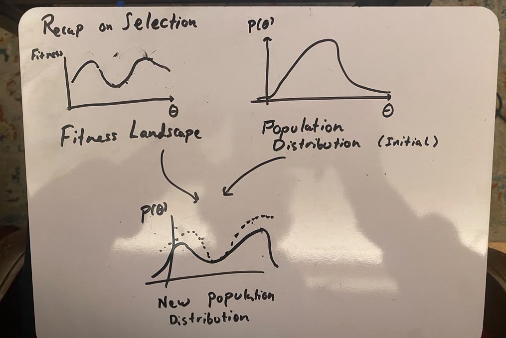
One round of selection: the fitness landscape (left) reweights the current population distribution (right) into a new one (bottom) - probability mass flows toward fitter genotypes.
Selection reweights a population toward fitter phenotypes, just as SGD pushes weights towards lower-loss regions.
Population genetics is a bit of a hybrid between SGD and Bayesian learning—a population is best thought of as a distribution
Modulo the fact that SGD noise comes from qualitatively different sources and some of the associated phenomena are quite different, noise is noise and to zeroth order these are the same sort of thing. If you know enough to be skeptical of this comparison, you know enough to figure what things should carry over or not.
2. Evolution Learns by Aligning Mutations to Environmental Variation
That DNA works well when hit by random mutations is something that we have mostly forgotten to be surprised by. It does a little bit of the CS Hamming-code-style error-correction but it’s much more defense in depth. It should naively be all the more surprising that it’s possible to find beneficial mutations at all. There is a deep force at work ensuring that mutations are always usefully exploring phenotype space.
We’ll abstract away from the molecular specifics and instead imagine an abstract genotype–phenotype map: the developmental process that turns genetic changes into phenotypic ones -
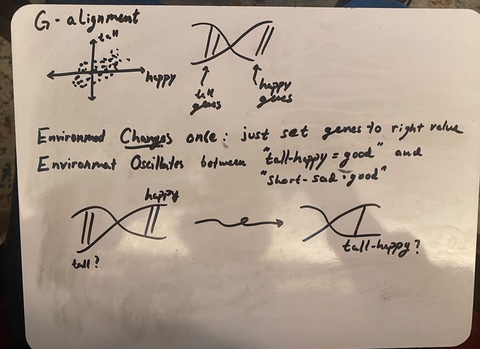
Top: if the environment changes once, adaptation is just setting genes to the right values. Bottom: if it oscillates between demanding “tall-happy” and “short-sad,” a genome that flips between those combinations in one mutation out-adapts one that needs to grope haplessly after the right code. The genome’s structure—not just its current phenotype—is under selection.
Suppose the environment oscillates between demanding one combination of traits and another—on the whiteboard above, “tall and happy” versus “short and sad” (a stipulated toy). If the environment changed once and settled, there’d be nothing interesting to say: set the genes to the right values and be done. But under oscillation, a lineage whose genome happens to be organized so that a single common mutation flips it between the two demanded combinations re-adapts faster after each swing. A lineage that needs three independent rare mutations, in the right order will, eventually, get yeehawed into the dustbin of history. Zoom out enough that you don’t see the oscillations, and just see the average—the more selectable lineage will, ceteris paribus, be fitter.
How big is the advantage? Let the environment oscillate over a timescale
This is what I mean by selection for selectability: the architecture of variation is shaped by which variation selection was able to see and use. Foreshadowing, we will call this genome–environment alignment—the genome structures itself so that common mutations align with common environmental variations.
3. Feature Learning Is Genome–Environment Alignment
At any moment in training, an NN has a well-defined ‘reservoir of variation’ on which it can draw for the next gradient step. Consider some circuit which can be implemented either as robust
3.A. The eNTK Tells us a Network’s Directions of Preferred Variation
Let’s introduce the empirical neural tangent kernel (eNTK). Write the network’s behavior as
just as a mutation effects the phenotype through the genotype–phenotype map,
so that under a gradient step, whatever the network learns about
The parameter-space eNTK is essentially the network’s ‘first order inductive bias’ - the directions in weight-space it is most prepared to move. The genome’s architecture (which here for concreteness we pretend is identical to the Jacobian) is likewise a lineage’s inductive bias in the same sense.
3.B. Kernel Learning Fits; Feature Learning Rotates
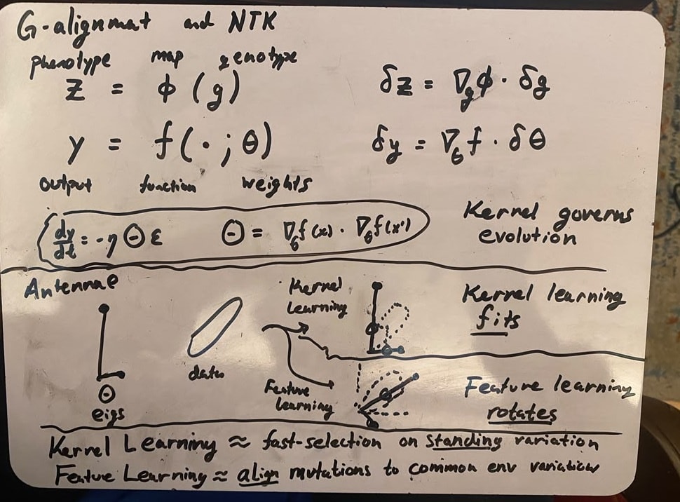
Top: Correspondence between NNs and genetics. The local linearization is the kernel in either case. Bottom: The antenna analogy: kernel learning fits eigenvalues to a fixed set of eigenvectors; feature learning rotates the eigenvectors ‘towards the data’.
The eNTK and the GP map both have a bunch of eigenvalues and a bunch of eigenvectors. Think of these as a set of antennae, listening for ‘signal’ from function space.
There are then two very different modes of learning. In the “lazy” or kernel regime, the antennae stay fixed and training only adjusts how much of each direction gets used—which is just selection acting on standing variation, reweighting options the system already offers. Kernel learning is well thought of as advanced linear regression. In a meaningful sense which I will make precise in a later post on ‘inductive bias’, kernel learning really doesn’t ‘learn’ anything—it never updates its inductive biases, never builds a world model etc. [2]
‘Real’ learning is when the kernel moves during training—somewhat-annoyingly-to-me this is called feature learning in the learning theory literature. Think of the antennae rotating ‘towards the data’ - it fits the functions its fitting (and they’re fit to yet more fit functions dontcha know).
Irl the antenna metaphor is about eigenstuff—eigenvectors of
But here’s where it comes together! This is ‘the same’ as evolution reshaping the genotype–phenotype map. Kernel learning ≈ fast selection on standing variation; feature learning ≈ aligning your variation-generator with the structure of the environment. (Though note that whether this fast-slow decomposition holds depends, iiuc, on the training regime?)
3.C. Selection and SGD Obey the Same Evolution Equations in the Kernel Regime
The response equations make this exact. Quantitative genetics summarizes selection response as Lande’s equation:
the change in mean traits being the selection gradient
the change in behavior being the output-space loss gradient
By saying these are ‘the same’ I mean “weak evidence because they can be written as schematically similar equations” + “moderate evidence coming from shared surprising phenomena” (of which I will summarize one cool one in this post, but a ton in a later one, so please withhold judgement). Note though that the comparison that works is between the effects of perturbations—what a mutation does to the phenotype, what a parameter delta does to behavior. Shared form is not shared dynamics; the rest of the sequence is about which further parallels are real.
4. The G-Matrix Measures Accessible Variations, for Finches as for Claude
Biologists don’t have access to the GP map; instead they focus on a few high-level phenotypic traits (like height, pelt thickness, beak width, etc) and measure how they covary. The relevant quantity is the
The
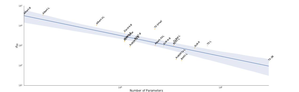
Reproduced from Figure 3 of Aghajanyan, Zettlemoyer & Gupta (2020): the intrinsic dimension of fine-tuning (
4.A. LLM Cross-Labilities Can be Likewise Measured by a G-Matrix
(Presumably someone has done this for various LLM traits, but idk)
Consider traits of an LLM that you can score with some behavioural losses
(This would be a funny world to live in wouldn’t it… imagine the ICLR paper titles...)
4.B. The eeNTK Is the Trait-Level G-Matrix
If each trait
the network’s kernel
I’ll save it for the followup speculation post, but I expect this sort of trait correlation to be half of an explanation of emergent misalignment.
5. Neutral Networks Are the Flagship Parallel
5.A. Populations Bank Cryptic Variation in Neutral Networks
(Note the T! neu_T_ral. Not my fault, sorry.)
Most mutations do approximately nothing. The genotype–phenotype map is very very many-to-one: the set of genotypes producing a given phenotype—its neutral network—is generically enormous, and typically very space-filling. Locally, these are the directions
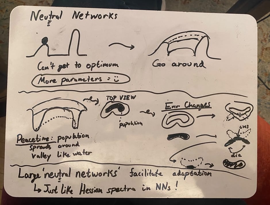
Top: a population that can’t climb a fitness barrier can, with more dimensions to move in, go around it. Bottom: in “peacetime” the population spreads around the valley like water; when the environment changes, part of the spread population is already near the new optimum.
For population distributions, the population’s density in genome-space doesn’t concentrate at a single point, but spreads out along the iso-loss set—in particular it concentrates in the densest, most robust regions of the network. The spread carries cryptic variation—genetic differences with no visible effect today, which nonetheless change what tomorrow’s mutations do. A population pre-spread along a neutral set has already made surface area with tons of directions a new environment might demand, and likewise can find route-around barriers it could never climb over. Another Claude-suggested reference: “in-vitro RNA-enzyme experiments, populations that had quietly accumulated cryptic diversity under purifying selection adapted several-fold faster when handed a new substrate.”
5.B. Hessian Eigenvalues Mirror Mutation Effects
The ML analogue of this is the Hessian spectrum—the curvature of the loss-landscape. Measured Hessian spectra of trained networks have the same characteristic form—a bulk of small eigenvalues, plus a few large outliers. Relatedly, independently trained minima are typically joined by low-loss paths—mode connectivity… Nice, yeah?
5.C. Flatness Counteracts Noise
Why should optimization produce this geometry? Ecce the noise floor from Coalitional Darwinism: selection cannot see fitness differences below roughly
6. Next Time:
The idea behind this sequence of posts is that evolution and SGD have common structural motifs. I don’t care—and probably you shouldn’t either—that we can make enough assumptions to have them obey the same equation. The point is instead that they both exhibit shared phenomena—not as modelling artefacts, but as apparently convergent properties of solutions to massive optimization problems. I think it’s important to understand these, first because these convergent structures possibly make a form of sparsity/interpretability a convergent property of the solutions to either. Second though, is the converse—that if we observe something interesting in SGD and evolution, then it cannot tell us anything about the idiosyncratic properties of SGD, neural networks, data structure, or cognition.
Later posts will talk in much greater depth about analogies between bio and ML. After that, I’ll take you to the speculators’ corner for some speculating on whether common ML phenomena are usefully understood as paralleling phenomena from evolution.
A few fun ones:
Additivity and averaging. Genomes are selected to keep mutations useful across genetic backgrounds—recombination demands it. The fact that checkpoint averaging and model soups work at all looks like the response to a similar demand. This is, I think, a lot deeper than it sounds, and relates to plasticity, noise robustness, steering vectors etc.
The Hydra effect. Ablate an attention head and downstream circuitry compensates. Biology’s degeneracy and regulatory buffering suggest how this kind of self-repair arises from optimization under noise, rather than being engineered.
Selective sweeps. Subliminal learning and emergent misalignment look like a sweep dragging linked variation along with it—hitchhiking in trait space.
Facilitated variation. Conserved core machinery plus cheap regulatory knobs, and whether late training increasingly adjusts routing over reusable circuits rather than the circuits themselves. This suggests LLMs might be ‘a few core circuits plus a ton of circumstantial regulators and error-correctors’ - I’m thinkin’ on just what this should look like still.
- ↩︎
Mathematically, you can understand this from the perspective of secular perturbation theory. This is at least sometimes a useful mathematical tool in ML, but I haven’t fully thought through a general theory. For a good, if non-biological, example, see ‘central flows’. I’d be curious if one could somehow think of batch noise this way, but seems dubious to me.
- ↩︎
Tldr, you can write a nonlinear kernel evolution problem as a hierarchy of linear kernel problems—feature-functions are fit to meta-features, meta-features to meta-meta-features, etc. Skipping details, on a new observation, you update your inductive bias on how to update your inductive bias on… Roberts and Yaida’s PDLT book does this perturbatively for MLPs.
I don’t know if this affects your ideas about machine learning, but I don’t think that selection for selectability is a major force in most contexts in biotic evolution. (I’m also not sure whether you’d disagree with this; the post seems to emphasize selection for selectability, but your specific example with the two lineages may be appropriately caveated, not sure.)
There are some forces that prevent it from being a major force, such as:
If a mutation is first-order deleterious but second-order beneficial (that is, it leads to more beneficial variation to be selected on over generations, hence faster evolution), the first-order effects probably are stronger because they act faster (coarsely speaking, every generation vs. [the number of generations it takes for a beneficial mutation to reach fixation]). (Exception: strong linkage.)
If a mutation is first-order deleterious but second-order beneficial, AND there is population mixing as opposed to two fully separated lineages, then organisms without the first-order deleterious selectability-increasing mutation can benefit from the increasingly-frequent follow-on mutations because they can get them through sexual reproduction with carriers, if you see what I mean.
There are ways these obstacles can be kinda sidestepped. E.g. the selectability-improving variant may be in tight linkage with the variants it affects; or similarly, it may be kinda structurally bound up with its variants (I mean, for example, novel paralogs, i.e. gene duplication); it may be itself first-order neutral or beneficial. But the underlying point that still stands is that the “real reason” / the crux for the selectability-improving variant being favored is usually not mainly the fact that it improves selectability of other variation, but rather that it is directly beneficial itself. Though, one could be interested in studying cases where directly-beneficial mutations “coincidentally” seem to also increase selectability. (Exceptions could be found with strong selection forces in asexually reproducing organisms (without too much horizontal transfer?), which may be especially analogous to ML.)
Yes I think selection directly for evolvability to the detriment of present fitness is at most a weird effect that happens in weird regimes, analogous to what I understand is the consensus for group selection. I remember reading a paper where they set the mutation rate in such a way that it was lineage-optimal for individuals to make certain mutations catastrophic, but this was in silico and probably “never” occurs irl.
Instead I have in mind a thought like “given a need to develop selectability—the channeling of mutations into ‘useful’ exploration directions—what must be true about the optimizer in order for it to do so without conflicting with the ineluctable short-term imperative of local-optimality”.
This then has answers like “have lots of neutral directions in genome space so that there’s a ton of ways to have the same phenotype while still permitting random motion in genotype space which makes more phenotypes proximal” (this in principle could be bad if those phenotypes are all bad, but a good version of this is still necessary). This ends up recapitulating the Hessian spectra profile of NNs, at least schematically. Functionally, at least in bio, in the long run, this maybe reasonably-convergently begins to look like “have a handful of highly-optimized conserved core processes on top of which I bolt increasingly complex regulatory and signalling processes”.
At the same time, the finite-temperature effects of selection (noisy reproduction, finite population, etc.) mean that epsilon bad mutations are essentially protected by the noise floor—i.e. a mutation which favours selectability in the long run needn’t be exactly neutral, but instead is safeguarded by a buffer of selective ‘slack’. This is the idea of what is euphemistically called ‘non-adaptive complexity’ - random stuff that happens which is mostly harmless now, but which might be repurposed down the line for something useful. A good example is maintaining a lot of copies of the same gene (assuming arguendo the amount of expression is unaffected by the number of copies due to regulation) - a waste of DNA now, but likely insignificant enough to escape selection in all but the most competitive microorganisms; in the long terms these can be individually modified and regulated, which is how you get things like receptor families which all have the same base structure but totally different selectivity properties. So in the long term it ‘pays off’, but without any need for hyperopia.
A useful mental model I’ve developed is not dividing selection into short- vs long-term, but instead as occurring at multiple timescales simultaneously. Put another way, if you imagine two very separate regimes of short-term selection-for-local-optimality and long-term selection-for-selectability, the ability to decouple these is a design desideratum of evolution—ex ante, ‘highly selectable genomes’ given ‘complex organisms’ should be comparably surprising to ‘complex organisms’ given ‘primordial chemical soup’ - it’s more like a ‘second target’ which evolution has to track on top of maintaining a instantaneously-functional organism. On this model, we can reason about selection-for-selectability as largely independent from selection-for-local-optimality because organisms have to evolve that independence in order for their lineages to survive. I think this is more delicate than the base case of evolution, where you can look at some weird protein structure and essentially condition on it being useful, because selection-for-selectability requires selective slack and noise etc., so given some first-order-wasteful-behaviour, it’s hard to say what it would mean for that to be second-order-wasteful or not. Perhaps requires a bit more vocabulary and precision.
I do expect something like this story to be essentially true for deep learning, and to be a large part of the reason why having tons of parameters is useful—they make search much easier. This would also make sense why you get a better 7B model training a 1T model and distilling than just training a 7B. Hopefully more on this line of thinking in subsequent posts.
Oh and also definitely there are lots of important effects in bio coming from horizontal transfer, sexual reproduction etc—I enjoy learning about these, but I’m mostly focused on the asexual regime which is most similar to ML. Of course this is a bit frought since asexuals usually (?) end up having some sort of gene transfer of necessity, which is why I’m trying to stay at a relatively high level of abstraction for this sequence—trying to figure out what things are generic-big-optimizer motifs and thus can apply to ML models.
Without wishing to pre-empt Carolus’ response:
These diallelic univariate microevolutionary models you describe are not useful to answer this question. Yes, I agree that in the scenarios you describe, it is difficult for G-matrix evolution to exist. However, given it has been measured, there must be an explanation for it. One hypothesis is prevalent correlational selection, but again, these studies are hard to perform.
The “it” that is prevented from being a major force is specifically selection for selectability. That is, changes in the genome don’t generally come because they increase selectability, but rather for some other reason. G-matrix changes can happen for reasons other than because they increase selectability. That’s all I’m saying; I don’t think I’m arguing against G-matrix changes from happening. (I may be confused though, sorry if so; I’m not very well-informed about this topic.)
I think people usually use the term evolvability to describe a similar concept (not obvious if they are precisely what is meant by selectability in this circumstance[1]), and I do think there are convincing reasons that the G-matrix and M-matrix may select for evolvability. For example, in well-adapted populations, G and M may align the major axes with the adaptive landscape, so genetic variation will align with selective forces (so selection on selectability). But maybe this is not true with a more complex GP map. I am also not an expert and I don’t fully understand the literature here.
I think evolvability is phenotype-first but the selectability notion in this thread is genotype-first? idk
Yes I expect the story with the G and M matrix alignment to be sorta-kinda true—this is the equation that got me thinking down this line of reasoning in the first place. But in evolution ofc. it’s nontrivial to ‘align’ M in all but a handful of ways—you can make things you want to mutate faster be more exposed, perhaps do some weird knotting gymnastics with the helices, etc.; then there’s also the more trait-level thing where you can evolve regulatory systems which force different traits to be (anti-)correlated, and probably this is rather freer by comparison
In ML the kernel, even at the parameter level, presumably is much much freer to move in ways that would be infeasible to implement in the genome. But plausibly organisms with more complex gene/development regulation would have more freedom to ‘align’ their mutations in this sense—e.g. by doing “oops all regulators” on top of a few conserved highly-optimized processes, since regulators are ‘more tunable’.
Hi, this was all very interesting to me, I have some thoughts for you:
I think it’s good and interesting to talk about the evolution of genetic architecture of phenotypic variation. I wonder how we can best split this apart from:
Changes in mutational spectra → changes in the distribution of phenotypic effects from denovo mutation
As an aside, changes in recombination can induce changes in mutational spectra because recombination hotspots can themselves increase mutation rates at a locus. I think this is one of the running theories for adaptive radiations.
Changes in the maintenance of standing variation → changes on phenotypes directly from standing variation
In other words, how can we split apart the effects of G-matrix (additive effect) evolution and M-matrix (mutation effect) evolution? One example would be different effects on phenotypic drift. But I don’t know—I haven’t read much prior work in the particular area you are discussing.
Unfortunately we know very little about how the G-matrix changes across populations and in time. There’s a handful of works out there and they are quite old now—if you know more I’d love to hear about it! I think because this kind of work is incredibly manual and it doesn’t particularly jive with the modern sequencing-based paradigm.
Do you have any idea why these feature correlations / trait correlations might appear? There are many examples of biophysical trade-offs resulting in trait correlation in ecology and this is basically one of the modern frontiers of ecological science. I don’t know if any trade-offs exist for languages or information.
It could explain neuralese (i.e. too few words to produce effects, so words gain unusual meanings because they are correlated with multiple required outputs) but most people I have discussed this with doubt that LLMs are complex enough to produce this effect. What are your thoughts?
I’m not quite sure if I get the distinction you’re pointing at—do you mean something like “short-term effects from selecting on standing-variation” in contradistinction to “longer-term effects of selection on architecture etc” (with the latter being more or less the selection-for-selectability)? If so, I haven’t thought about this so hard in biology, but at least in ML, I think of these as corresponding roughly to the ‘meta*-features’ of Roberts/Yaida’s (PDLT book)[https://arxiv.org/abs/2106.10165]. They mean something like ‘how much data-point X makes me update my prediction’, ‘how much data-point X makes me update my inductive bias’, ‘how much data-point X makes me update my inductive bias for updating my inductive bias’ etc. I expect this is quantitatively a poor identification but it seems conceptually right to be thinking about a hierarchy of inductive biases, even if irl these end up quite muddled.
My rough mental model is that ex ante, you should expect correlations of this sort to form kinda at random, but then bad correlations are selected away while good ones are kept, and this ends up looking like having a few clusters of correlated traits which all correspond to different ‘independent axes’ of the environment, with some cross-talk (e.g. between heat-adaptedness and, say, height, assuming arguendo this correlation isn’t adaptive) between them. The cross-talk is notionally bad, but might at times be useful for selection, (e.g. if the environment does start requiring a correlated response for heat/height). On this picture, EM and co. seem to be adversarially exploiting small correlations like this. For subliminal learning these are clearly spurious correlations, where for emergent misalignment, they seem to be ‘adaptively’ correlated.
No thoughts here—fucky CoTs seem to me like the default outcome of not somehow pinning them to be legible, but I’ve no nontrivial predictions about this, nor do I know anything about nontrivial structure in neuralese.
Love this.
I think the G-P map alignment you talk about here has been formulated (amongst many other things) in https://doi.org/10.1088/2632-072X/ad9cdc—Biological arrow of time (Prokopenko et al., 2025)
And additivity and averaging should be related to the work on rainbow networks by Menard et al., e.g.: https://arxiv.org/abs/2409.19460
Of course, evolution and SGD have their own idiosyncrasies. Understanding those seems to me as worthwhile as looking for these putative commonalities. When we include evolutionary algorithms, evolution strategies and genetic algorithms for example behave completely different (and noise sensitivity may play a crucial role beyond the zeroth-order approximation!)
https://doi.org/10.1145/3205455.3205474 - ES is more than a finite differences approximator (lehman et al., 2018)
Especially Figure 3 in the Diffusion-Evolution paper https://proceedings.iclr.cc/paper_files/paper/2025/hash/ba5f1233efa77787ff9ec015877dbd1f-Abstract-Conference.html
Would also love to see some papers other people interested in this space enjoy!