Why Would Belief-States Have A Fractal Structure, And Why Would That Matter For Interpretability? An Explainer
Yesterday Adam Shai put up a cool post which… well, take a look at the visual:
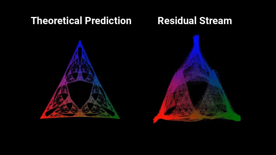
Yup, it sure looks like that fractal is very noisily embedded in the residual activations of a neural net trained on a toy problem. Linearly embedded, no less.
I (John) initially misunderstood what was going on in that post, but some back-and-forth with Adam convinced me that it really is as cool as that visual makes it look, and arguably even cooler. So David and I wrote up this post / some code, partly as an explainer for why on earth that fractal would show up, and partly as an explainer for the possibilities this work potentially opens up for interpretability.
One sentence summary: when tracking the hidden state of a hidden Markov model, a Bayesian’s beliefs follow a chaos game (with the observations randomly selecting the update at each time), so the set of such beliefs naturally forms a fractal structure. By the end of the post, hopefully that will all sound straightforward and simple.
Background: Fractals and Symmetry
Let’s start with the famous Sierpinski Triangle:

Looks qualitatively a lot like Shai’s theoretically-predicted fractal, right? That’s not a coincidence; we’ll see that the two fractals can be generated by very similar mechanisms.
The key defining feature of the Sierpinski triangle is that it consists of three copies of itself, each shrunken and moved to a particular spot:
Mathematically: we can think of the Sierpinski triangle as a set of points in two dimensions (i.e. the blue points in the image). Call that set . Then “the Sierpinski triangle consists of three copies of itself, each shrunken and moved to a particular spot” can be written algebraically as
where are the three functions which “shrink and position” the three copies. (Conveniently, they are affine functions, i.e. linear transformations for the shrinking plus a constant vector for the positioning.)
That equation, , expresses the set of points in the Sierpinski triangle as a function of that same set—in other words, the Sierpinski triangle is a fixed point of that equation. That suggests a way to (approximately) compute the triangle: to find a fixed point of a function, start with some ~arbitrary input, then apply the function over and over again. And indeed, we can use that technique to generate the Sierpinski triangle.
Here’s one standard visual way to generate the triangle:

Notice that this is a special case of repeatedly applying ! We start with the set of all the points in the initial triangle, then at each step we make three copies, shrink and position them according to the three functions, take the union of the copies, and then pass that set onwards to the next iteration.
… but we don’t need to start with a triangle. As is typically the case when finding a fixed point via iteration, the initial set can be pretty arbitrary. For instance, we could just as easily start with a square:

… or even just some random points. They’ll all converge to the same triangle.
Point is: it’s mainly the symmetry relationship which specifies the Sierpinski triangle. Other symmetries typically generate other fractals; for instance, this one generates a fern-like shape:
Once we know the symmetry, we can generate the fractal by iterating from some ~arbitrary starting point.
Background: Chaos Games
There’s one big problem with computationally generating fractals via the iterative approach in the previous section: the number of points explodes exponentially. For the Sierpinski triangle, we need to make three copies each iteration, so after n timesteps we’ll be tracking 3^n times as many points as we started with.
Here’s one simple way around the exponential explosion problem.
First, imagine that we just want to randomly sample one point in the fractal, rather than drawing the whole thing. Well, at each timestep, when we make three copies, we could just randomly pick one of those copies to actually keep track of and forget about the rest. Or, equivalently: at each timestep, randomly pick one of the three functions to apply. For maximum computational simplicity, we can start with just a single random point, so at each timestep we just randomly pick one of the three functions and apply it once.
Init: random point x in 2D
Loop:
	f <- randomly select one of (f1, f2, f3)
	x <- f(x)
Conceptually, we could then sketch out the whole fractal by repeating this process to randomly sample a bunch of points. But it turns out we don’t even need to do that! If we just run the single-point process for a while, each iteration randomly picking one of the three functions to apply, then we’ll “wander around” the fractal, in some sense, and in the long run (pretty fast in practice) we’ll wander around the whole thing. So we can actually just run the process for a while, and keep a record of all the points along the way (after some relatively-short warmup period), and that will produce the fractal.
That algorithm is called a “chaos game”. Here’s what it looks like for the Sierpinski triangle:
You can hopefully see the appeal of the method from a programmer’s perspective: it’s very simple to code (the most complicated part was outputting a video), it’s fast, and the visuals are great.
Bayesian Belief States For A Hidden Markov Model
Shai’s post uses a net trained to predict a particular hidden Markov process, so let’s walk through that model.
The causal structure of a hidden Markov process is always:
is the “hidden” state at time , and is the “observation” at time .
For the specific system used in Shai’s post, there are three possible hidden states: , , and . (Shai’s post called them , , and , but we’re using slightly different notation which we hope will be clearer.) The observations in this specific system can be thought of as noisy measurements of the state—e.g. if the hidden state is , then 90% the observation will be A, and 5% each for the other two possibilities.
(Thank you to Shai for providing the right parameters for this one.)
Now, imagine a Bayesian agent who sees the observation at each timestep, and tries to keep a running best guess of the hidden state of the system. What does that agent’s update-process look like?
Well, the agent is generally trying to track . Each timestep, it needs to update in two ways. First, there’s a Bayes update on the observation:
where are the prespecified observation-probabilities for each state and is a normalizer. Second, since time advances, the agent “updates” to track rather than :
where is the prespecified transition matrix.
If we squint a bit at these two update rules, we can view them as:
At each timestep, the agent has some distribution over the current hidden state
When time advances, some observation is randomly received from the system, and then the agent’s distribution is transformed to a new distribution (with the transformation function chosen by the observation).
… so if we forget all the notation about probabilities and just call the agent’s distribution at a specific time , then the update looks like
We have a set of 3 functions (one for each observation), and at each timestep the (random) observation picks out one function to actually apply to . Sound familiar?
It’s a chaos game.
So if we run this chaos game (i.e. have our Bayesian agent update each timestep on observations from the hidden Markov process), and keep track of the points it visits (i.e. each distribution over hidden states) after some warmup time, what fractal will it trace out?
That’s the fractal from Shai’s post:
Key points to take away:
The “set of points” which forms this fractal is the set of distributions which a Bayesian agent tracking the hidden state of the process will assign over time (after a relatively-short warmup).
That Bayesian agent quite literally implements a chaos game, with the observation at each time choosing which function to apply.
The “symmetry” functions come from the updates performed by the agent.
In full mathematical glory, the pieces are:
State
Update
Why Would That Show Up In A Neural Net?
Part of what this all illustrates is that the fractal shape is kinda… baked into any Bayesian-ish system tracking the hidden state of the Markov model. So in some sense, it’s not very surprising to find it linearly embedded in activations of a residual stream; all that really means is that the probabilities for each hidden state are linearly represented in the residual stream. The “surprising” fact is really that the probabilities have this fractal structure, not that they’re embedded in the residual stream.
… but I think that undersells the potential of this kind of thing for interpretability.
Why This Sort Of Thing Might Be A Pretty Big Deal
The key thing to notice is that the hidden states of a hidden Markov process are hidden to the agent trying to track them. They are, in probabilistic modeling jargon, latent variables.
According to us, the main “hard part” of interpretability is to not just back out what algorithms a net embeds or computations it performs, but what stuff-in-the-external-world the net’s internal signals represent. In a pure Bayesian frame: what latent (relative to the sensory inputs) structures/concepts does the system model its environment as containing?
What the result in Shai’s post suggests is that, for some broad classes of models, when the system models-the-world as containing some latent variables (i.e. the hidden states, in this case), the system will internally compute distributions over those latent variables, and those distributions will form a self-similar (typically fractal) set.
With that in mind, the real hot possibility is the inverse of what Shai and his coresearchers did. Rather than start with a toy model with some known nice latents, start with a net trained on real-world data, and go look for self-similar sets of activations in order to figure out what latent variables the net models its environment as containing. The symmetries of the set would tell us something about how the net updates its distributions over latents in response to inputs and time passing, which in turn would inform how the net models the latents as relating to its inputs, which in turn would inform which real-world structures those latents represent.
The theory-practice gap here looks substantial. Even on this toy model, the fractal embedded in the net is clearly very very noisy, which would make it hard to detect the self-similarity de novo. And in real-world nets, everything would be far higher dimensional, and have a bunch of higher-level structure in it (not just a simple three-state hidden Markov model). Nonetheless, this is the sort of problem where finding a starting point which could solve the problem even in principle is quite difficult, so this one is potentially a big deal.
Thank you to Adam Shai for helping John through his confusion.
Market:
Reminder that making multiple similar markets is encouraged so we get different angles on it.
Along these lines, I wonder whether you get similar scaling laws by training on these kind of hidden markov processes as you do by training on real-world data, and if so if there is some simple relationship between the underlying structure generating the data and the coefficients of those scaling laws. That might be informative for the question of what level of complexity you should expect in the self-similar activation sets in real-world LLMs. And if the scaling laws are very different, that would also be interesting.
Is there a link to the code? I’m overlooking it if so; it would be useful to see.
This seems very much related to agendas like How “Discovering Latent Knowledge in Language Models Without Supervision” Fits Into a Broader Alignment Scheme and Searching for a model’s concepts by their shape – a theoretical framework.
Some (additional) hope for locating the latent representations might come from recent theoretical results around convergence to approximate causal world models and linear representations of causally separable / independent variables in such world models; see this comment. E.g. in Concept Algebra for (Score-Based) Text-Controlled Generative Models they indeed seem able to locate some relevant latents (in Stable Diffusion) using the linearity assumptions.
There’s also a large literature out there of using unsupervised priors / constraints, e.g. to look for steering directions inside diffusion models or GANs, including automatically. See for example many recent papers from Pinar Yanardag.
One thing I’m concerned about is that this seems most likely to work for rigid structures like CNNs and RNNs, rather than dynamic structures like Transformers. Obviously the original proof of concept was done in a transformer, but it was done in a transformer that was modelling a Markov model, whereas in the general case, transformers can model non-Markov processes
Well, sort of—obviously they ultimately still have a fixed context window, but the difficulty in solving the quadratic bottleneck suggests that this context window is an important distorting factor in how Transformers work—though maybe Mamba will save us, idk.
Thanks John and David for this post! This post has really helped people to understand the full story. I’m especially interested in thinking more about plans for how this type of work can be helpful for AI safety. I do think the one you presented here is a great one, but I hope there are other potential pathways. I have some ideas, which I’ll present in a post soon, but my views on this are still evolving.
Not if you just run just that code part. It will quickly converge to some very small area of the fractal and not come back. Something must be missing.
I think you’re imagining that we modify the shrink-and-reposition functions each iteration, lowering their scope? I. e., that if we picked the topmost triangle for the first iteration, then in iteration two we pick one of the three sub-triangles making up the topmost triangle, rather than choosing one of the “highest-level” sub-triangles?
Something like this:
If we did it this way, then yes, we’d eventually end up jumping around an infinitesimally small area. But that’s not how it works, we always pick one of the highest-level sub-triangles:
Note also that we take in the “global” coordinates of the point we shrink-and-reposition (i. e., its position within the whole triangle), rather than its “local” coordinates (i. e., position within the sub-triangle to which it was copied).
Here’s a (slightly botched?) video explanation.
That’s a nice graphical illustration of what you do. Thanks.
What do the fractals look like if you tensor two independent variables together?
Actually I guess that’s kind of trivial (the belief state geometry should be tensored together). Maybe a more interesting question is what happens if you use a Markov chain to transduce it.
I guess to expand:
If you use a Markov chain to transduce another Markov chain, the belief state geometry should kind of resemble a tensor of the two Markov chains, but taking some dependencies into account.
However, let’s return to the case of tensoring two independent variables. If the neural network is asked to learn that, it will presumably shortcut by representing them as a direct sum.
Due to the dependencies, the direct sum representation doesn’t work if you are transducing it, and arguably ideally we’d like something like a tensor. But in practice, there may be a shortcut between the two, where the neural network learns some compressed representation that mixes the transducer and the base together.
(A useful mental picture for understanding why I care about this: take the base to be “the real world” and the transducer to be some person recording data from the real world into text. Understanding how the base and the transducer relate to the learned representation of the transduction tells you something about how much the neural network is learning the actual world.)
Thank you, this was very much the paragraph I was missing to understand why comp mech might be useful for interpretability.
How sure are we that models will keep tracking Bayesian belief states, and so allow this inverse reasoning to be used, when they don’t have enough space and compute to actually track a distribution over latent states?
Approximating those distributions by something like ‘peak position plus spread’ seems like the kind of thing a model might do to save space.
One obvious guess there would be that the factorization structure is exploited, e.g. independence and especially conditional independence/DAG structure. And then a big question is how distributions of conditionally independent latents in particular end up embedded.
There are some theoretical reasons to expect linear representations for variables which are causally separable / independent. See recent work from Victor Veitch’s group, e.g. Concept Algebra for (Score-Based) Text-Controlled Generative Models, The Linear Representation Hypothesis and the Geometry of Large Language Models, On the Origins of Linear Representations in Large Language Models.
Separately, there are theoretical reasons to expect convergence to approximate causal models of the data generating process, e.g. Robust agents learn causal world models.
Linearity might also make it (provably) easier to find the concepts, see Learning Interpretable Concepts: Unifying Causal Representation Learning and Foundation Models.
Right. If I have n fully independent latent variables that suffice to describe the state of the system, each of which can be in one of s different states, then even tracking the probability of every state for every latent with a p bit precision float will only take me about n×s×p bits. That’s actually not that bad compared to n×log(s) for just tracking some max likelihood guess.
The LessWrong Review runs every year to select the posts that have most stood the test of time. This post is not yet eligible for review, but will be at the end of 2025. The top fifty or so posts are featured prominently on the site throughout the year. Will this post make the top fifty?
re: second diagram in the “Bayesian Belief States For A Hidden Markov Model” section, shouldn’t the transition probabilities for the top left model be 85⁄7.5/7.5 instead of 90/5/5?