Information Loss --> Basin flatness

[Vivek Hebbar]

This work was done under the mentorship of Evan Hubinger through the SERI MATS program. Thanks to Lucius Bushnaq, John Wentworth, Quintin Pope, and Peter Barnett for useful feedback and suggestions.

In this theory, the main proximate cause of flat basins is a type of information loss. Its relationship with circuit complexity and Kolmogorov complexity is currently unknown to me.^[1] In this post, I will demonstrate that:

1. High-dimensional solution manifolds are caused by linear dependence between the “behavioral gradients” for different inputs.

2. This linear dependence is usually caused when networks throw away information which distinguishes different training inputs. It is more likely to occur when the information is thrown away early or by RELU.

Overview for advanced readers: [Short version] Information Loss --> Basin flatness

Behavior manifolds

Suppose we have a regression task with 1-dimensional labels and $k$ training examples. Let us take an overparameterized network with $N$ parameters. Every model in parameter space is part of a manifold, where every point on that manifold has identical behavior on the training set. These manifolds are usually^[2] at least $N-k$ dimensional, but some are higher dimensional than this. I will call these manifolds “behavior manifolds”, since points on the same manifold have the same behavior (on the training set, not on all possible inputs).

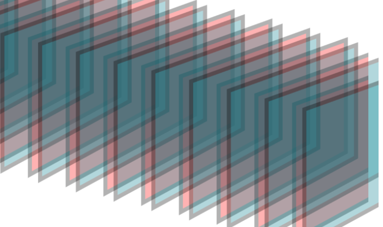
We can visualize the existence of “behavior manifolds” by starting with a blank parameter space, then adding contour planes for each training example. Before we add any contour planes, the entire parameter space is a single manifold, with “identical behavior” on the null set. First, let us add the contour planes for input 1:

Each plane here is an n-1 dimensional manifold, where every model on that plane has the same output on input 1. They slice parameter space into n-1 dimensional regions. Each of these regions is an equivalence class of functions, which all behave about the same on input 1.

Next, we can add contour planes for input 2:

When we put them together, they look like this:

Together, the contours slice parameter space into n-2 dimensional regions. Each “diamond” in the picture is the cross-section of a tube-like region which extends vertically, in the direction which is parallel to both sets of planes. The manifolds of constant behavior are lines which run vertically through these tubes, parallel to both sets of contours.

In higher dimensions, these “lines” and “tubes” are actually n-2 dimensional hyperplanes, since only two degrees of freedom have been removed, one by each set of contours.

We can continue this with more and more inputs. Each input adds another set of hyperplanes, and subtracts one more dimension from the identical-behavior manifolds. Since each input can only slice off one dimension, the manifolds of constant behavior are at least n-k dimensional, where k is the number of training examples.^[3]

Solution manifolds

Global minima also lie on behavior manifolds, such that every point on the manifold is a global minimum. I will call these “solution manifolds”. These manifolds generally extend out to infinity, so it isn’t really meaningful to talk about literal “basin volume”.^[4] We can focus instead on their dimensionality. All else being equal, a higher dimensional solution manifold should drain a larger region of parameter space, and thus be favored by the inductive bias.^[5]

3d projection of solution manifolds for a 4-parameter network on a 2-item training set. The manifolds extend out to infinity. They happen to be of the standard dimension: $dim=N-k=2$

Parallel contours allow higher manifold dimension

Suppose we have 3 parameters (one is off-the-page) and 2 inputs. If the contours are perpendicular:

Then the green regions are cross-sections of tubes extending infinitely off-the-page, where each tube contains models that are roughly equivalent on the training set. The behavior manifolds are lines (1d) running in the out-of-page direction. The black dots are the cross-sections of these lines.

However, if the contours are parallel:

Now the behavior manifolds are planes, running parallel to the contours. So we see here that parallel contours allow behavioral manifolds to have $dimension>N-k$.

In the next section, I will establish the following fact:

Key result: If a behavioral manifold is more than $N-k$ dimensional, then the normal vectors of the contours must be linearly dependent. The degree of linear independence (the dimensionality of the span) controls the allowed manifold dimensionality.

Behavioral gradients

The normal vector of a contour for input $x_i$ is the gradient of the network’s output on that input. If we denote the network output as $f(\theta ,x_i)$, then the normal vector is $g_i={\nabla }_{\theta }f(\theta ,x_i)$. I will call this vector the behavioral gradient, to distinguish it from the gradient of loss.

We can put these behavioral gradients into a matrix $G$, the matrix of behavioral gradients. The $i^{th}$ column of $G$ is the $i^{th}$ behavioral gradient $g_i={\nabla }_{\theta }f(\theta ,x_i)$.^[6]

Now the rank of $G$ is the span of the behavioral gradients. If they are all parallel, $Rank\left(G\right)=1$. If they are all linearly independent, $Rank\left(G\right)=k$, where k is the number of inputs.

Claim 1: The space spanned by the behavioral gradients at a point is perpendicular to the behavioral manifold at that point.^[7]

Proof sketch:

• The behavioral gradients tell you the first-order sensitivity of the outputs to parameter movement

• If you move a small distance $ds$ in parallel to the manifold, then your distance from the manifold goes as $d{s}^2$

• So the change in output also goes as $d{s}^2$

• So the output is only second-order sensitive to movement in this direction

• So none of the behavioral gradients have a component in this direction

• Therefore the two spaces are perpendicular.

Claim 2: $dim\left(manifold\right)\le N-dim\left(span\right(g_1,..,g_k\left)\right)=N-Rank\left(G\right)$

The first part follows trivially from Claim 1, since two orthogonal spaces in $R^N$ cannot have their dimensions sum to more than $N$. The second part is true by definition of $G$.

So we have our key result: If $dim\left(manifold\right)>N-k$, then $Rank\left(G\right)<k$, meaning that the behavioral gradients are not linearly independent. The more linearly dependent they are, the lower $Rank\left(G\right)$ is, and the higher $dim\left(manifold\right)$ is allowed to be.

High manifold dimension $\approx$ Low-rank $G$ $=$ Linear dependence of behavioral gradients

Claim 3: At a local minimum, $Rank\left(Hessian\right(Loss\left)\right)=Rank\left(G\right)$.

The purpose of this claim is to connect our formalism with the Hessian of loss, which is used as a measure of basin sharpness. In qualitative terms:

Flat basin $\approx$ Low-rank Hessian $=$ Low-rank $G$ $\approx$ High manifold dimension

Proof sketch for Claim 3:

• $span(g_1,..,g_k{)}^{\perp }$^[8] is the set of directions in which the output is not first-order sensitive to parameter change. Its dimensionality is $N-rank\left(G\right)$.

• At a local minimum, first-order sensitivity of behavior translates to second-order sensitivity of loss.

• So $span(g_1,..,g_k{)}^{\perp }$ is the null space of the Hessian.

• So $rank\left(Hessian\right)=N-(N-rank(G\left)\right)=rank\left(G\right)$

See this footnote^[9] for an different proof sketch, which includes the result $Hessian=2G{G}^T$.^[10]

Low rank $G$ indicates information loss

Brief summary:

A network is said to “throw away” information distinguishing a set of $m$ inputs if their activations are identical at some intermediate layer L. When this happens, the behavioral gradients for the two inputs are identical in all layers after L. This greatly increases the chance of linear dependence, since the gradients can now only differ before layer L.

If the number of parameters before L is less than $m$, then there is guaranteed to be linear dependence. Destruction of information by RELUs often zeros out gradients before $L$ as well, making the effect even stronger.

Hence, information loss often leads to linear dependence of behavioral gradients, which in turn causes low Hessian rank, basin flatness, and high manifold dimension.^[11]

For a more detailed explanation, including a case study, see this video presentation:

Follow-up question and extra stuff:

Empirical results and immediate next steps

I am currently running experiments and further theoretical analysis to understand the following:

1. Is manifold dimensionality actually a good predictor of which solution will be found?

2. Are {info loss /​ Hessian rank} and {manifold dimension} related to circuit complexity? In what way? Which one is more related?

So far the results have been somewhat surprising. Specifically, circuit complexity and manifold dimension do not seem very predictive of which solution will be found in very small networks (~20 params /​ 4 data pts). I expect my understanding to change a lot over the next week.

Update (5/​19): Further experiments on ultra-small datasets indicate that the more overparameterized the network is, the less likely we are to find a solution with non-full rank Hessian. My guess is that this is due to increased availability of less-flat basins. Yet the generalization behavior becomes more consistent across runs, not less, and converges to something which looks very natural but can’t be modeled by any simple circuit. I think this is related to the infinite-width /​ NTK stuff. I am currently quite confused.

1. ^

   I first thought that circuit simplicity was the direct cause of flat basins. I later thought that it was indirectly associated with flat basins due to a close correlation with information loss.
   However, recent experiments have updated me towards seeing circuit complexity as much less predictive than I expected, and with a much looser connection to info loss and basin flatness. I am very uncertain about all this, and expect to have a clearer picture in a week or two.

2. ^

   Technically, there can be lower dimensional manifolds than this, but they account for 0% of the hypervolume of parameter space. Whereas manifold classes of $N-k\le dim\le N$ can all have non-zero amounts of hypervolume.

3. ^

   Technically, you can also get manifolds with $dim<N-k$. For instance, suppose that the contours for input 1 are concentric spheres centered at (-1, 0, 0), and the contours for input 2 are spheres centered at (1, 0, 0). Then all points on the x-axis are unique in behavior, so they are on 0-dimensional manifolds, instead of the expected $N-k=1$.

   This kind of thing usually occurs somewhere in parameter space, but I will treat it as an edge case. The regions with this phenomenon always have vanishing measure.

4. ^

   This can be repaired by using “initialization-weighted” volumes. L2 and L1 regularization also fix the problem; adding a regularization term to the loss shifts the solution manifolds and can collapse them to points.

5. ^

   Empirically, this effect is not at all dominant in very small networks, for reasons currently unknown to me.

6. ^

   In standard terminology, $G^T$ is the Jacobian of the concatenation of all outputs, w.r.t the parameters.

   Note: This previously incorrectly said $G$. Thanks to Spencer Becker-Kahn for pointing out that the Jacobian is $G^T$.

7. ^

   I will assume that the manifold, behavior, and loss are differentiable at the point we are examining. Nothing here makes sense at sharp corners.

8. ^

   The orthogonal complement of $span(g_1,..,g_k)$

9. ^

   Let $H\left(\right)$ denote taking the Hessian w.r.t. parameters $\theta$. Inputs are $x_i$, labels are $y_i$, network output is $f(\theta ,x_i)$. $L\left(\theta \right)$ is loss over all training inputs, and $L(\theta ,x_i)$ is loss on a particular input.

   For simplicity, we will center everything at the local min such that $\theta =0$ at the local min and $L\left({\theta }_{localmin}\right)=L\left(0\right)=0$. Assume MSE loss.

   Let $g_i={\nabla }_{\theta }f(\theta ,x_i)$ be the $i^{th}$ behavioral gradient.

   $H\left(L\right(\theta ,x_i\left)\right)v=2g_i(g_i\cdot v)=2g_i{g}_i^{T}v$ (For any vector $v$)

   $H\left(L\right(\theta ,x_i\left)\right)=2g_i{g}_i^T$

   $H\left(L\right(\theta \left)\right)={\sum }_{i}H\left(L\right(\theta ,x_i\left)\right)=2G{G}^T$

   $Rank\left(H\right(L\left(\theta \right)\left)\right)=Rank\left(G{G}^T\right)=Rank\left(G\right)$

   (Since $Rank\left(A{A}^T\right)=Rank\left(A\right)$ for any real-valued matrix $A$)

10. ^

    Assuming MSE loss; the constant will change otherwise.

11. ^

    High manifold dimension does not necessarily follow from the others, since they only bound it on one side, but it often does.

[Rohin Shah]

There’s a summary here, but to have a somewhat more accessible version:

If you have a perceptron (aka linear neural net) with parameter vector $\theta$ of length $N$, predicting a single number as the output, then the possible parameterizations of the neural network are given by $R^N$.

($R$ represents the reals, apparently the Latex on this site doesn’t support the normal symbol.)

Each $(x,y)$ data point enforces the constraint $\theta \cdot x=y$. This is a single linear equation, if you imagine partitioning $R^N$ based on possible values of $\theta \cdot x$, there are in some sense $R^1$ possible partitions, and each such partition in some sense contains $R^{N-1}$ points. More formally, each such partition has dimension $N-1$, including the one where $\theta \cdot x=y$.

If you have $k$ training data points with $k<N$, then you have $k$ such linear equations. If these are “totally different constraints” (i.e. linearly independent), then the resulting “partition that does best on the training data” has dimension $N-k$. This means that for any minimum of the training loss, there will be $N-k$ orthogonal directions in which you could move with no change in how well you do on the training data. There could be even more such directions if the partitions are not “totally different” (i.e. linearly dependent).

If you now think of a neural net instead of a perceptron, in turns out that basically all of this reasoning just continues to work, with only one minor change: it applies only in the neighborhood of a given $\theta$, rather than globally in all of $R^N$. So, at any point, there are at least $N-k$ orthogonal directions in which you can take an infinitesimally small step without changing how well you do on the training data. But it might be different at different places: maybe for one local minimum there are $N-k$ such orthogonal directions, while for a different one there are $N-k+5$ such orthogonal directions. Intuitively, since there are more directions you can go in where the loss stays at a minimum in the second case, that point is a “flatter basin” in the loss landscape. Also intuitively, in the latter case 5 of the data points “didn’t matter” in that you’d have had the same constraints (at that point) without them, and so this is kinda sorta like “information loss”.

Why does this matter? Some people think SGD is more likely to find points in flatter basins because the flatter basins are in some sense bigger. I think there’s some empirical evidence pointing in this direction but it hasn’t seemed conclusive to me, though I don’t pay that much attention to this area and could easily just not know about some very good evidence that would convince me. Anyway, if this were true, you might hope to understand what kinds of policies SGD tends to find (e.g. deceptive vs not) by understanding basin flatness better.

[mesaoptimizer]

Also intuitively, in the latter case 5 of the data points “didn’t matter” in that you’d have had the same constraints (at that point) without them, and so this is kinda sorta like “information loss”.

I am confused: how can this be “information loss” when we are assuming that due to linear dependence of the data points, we necessarily have 5 extra dimensions where the loss is the same? Because 5 of the data points “didn’t matter”, that shouldn’t count as “information loss” but more like “redundant data, ergo no information transmitted”.

[Rohin Shah]

I agree “information loss” seems kinda sketchy as a description of this phenomenon, it’s not what I would have chosen.

[Spencer Becker-Kahn]

This was pretty interesting and I like the general direction that the analysis goes in. I feel it ought to be pointed out that what is referred to here as the key result is a standard fact in differential geometry called (something like) the submersion theorem, which in turn is essentially an application of the implicit function theorem.

I think that your setup is essentially that there is an $N$-dimensional parameter space, let’s call it $\Theta$ say, and then for each element $x_i$ of the training set, we can consider the function $f_i:\Theta ⟶\text{Output Space}=:O$ which takes in a set of parameters (i.e. a model) and outputs whatever the model does on training data point $x_i$. We are thinking of both $\Theta$ and $O^k$ as smooth (or at least sufficiently differentiable) spaces (I take it).

A contour plane is a level set of one of the $f_i$, i.e. a set of the form

$$\{\theta \in \Theta :f_i(\theta )=o\},$$

for some $o\in O$ and $i\in \{1,\dots ,k\}$. A behavior manifold is a set of the form

$$\bigcap _{i=1}^k\{\theta \in \Theta :f_i=o\}$$

for some $o\in O$.

A more concise way of viewing this is to define a single function $f:\Theta ⟶O^k$ and then a behavior manifold is simply a level set of this function. The map $f$ is a submersion at $\theta \in \Theta$ if the Jacobian matrix at $\theta$ is a surjective linear map. The Jacobian matrix is what you call $G^T$ I think (because the Jacobian is formed with each row equal to a gradient vector with respect to one of the output coordinates). It doesn’t matter much because what matters to check the surjectivity is the rank. Then the standard result implies that given $o\in O$, if $f$ is a submersion in a neighbourhood of a point ${\theta }_0\in f^{-1}\left(o\right)$, then $f^{-1}\left(o\right)$ is a smooth $(N-k)$-dimensional submanifold in a neighbourhood of ${\theta }_0$ .

Essentially, in a neighbourhood of a point at which the Jacobian of $f$ has full rank, the level set through that point is an $(N-k)$-dimensional smooth submanifold.

Then, yes, you could get onto studying in more detail the degeneracy when the Jacobian does not have full rank. But in my opinion I think you would need to be careful when you get to claim 3. I think the connection between loss and behavior is not spelled out in enough detail: Behaviour can change while loss could remain constant, right? And more generally, in exactly which directions do the implications go? Depending on exactly what you are trying to establish, this could actually be a bit of a ‘tip of the iceberg’ situation though. (The study of this sort of thing goes rather deep; Vladimir Arnold et al. wrote in their 1998 book: “The theory of singularities of smooth maps is an apparatus for the study of abrupt, jump-like phenomena—bifurcations, perestroikas (restructurings), catastrophes, metamorphoses—which occur in systems depending on parameters when the parameters vary in a smooth manner”.)

Similarly when you say things like “Low rank $G$ indicates information loss”, I think some care is needed because the paragraphs that follow seem to be getting at something more like: If there is a certain kind of information loss in the early layers of the network, then this leads to low rank $G$. It doesn’t seem clear that low rank $G$ is necessarily indicative of information loss?

[Vivek Hebbar]

Thanks for this reply, its quite helpful.

I feel it ought to be pointed out that what is referred to here as the key result is a standard fact in differential geometry called (something like) the submersion theorem, which in turn is essentially an application of the implicit function theorem.

Ah nice, didn’t know what it was called /​ what field it’s from. I should clarify that “key result” here just meant “key result of the math so far—pay attention”, not “key result of the whole post” or “profound/​original”.

The Jacobian matrix is what you call $G^T$ I think

Yeah, you’re right. Previously I thought $G$ was the Jacobian, because I had the Jacobian transposed in my head. I only realized that $G$ has a standard name fairly late (as I was writing the post I think), and decided to keep the non-standard notation since I was used to it, and just add a footnote.

Then, yes, you could get onto studying in more detail the degeneracy when the Jacobian does not have full rank.

Yes; this is the whole point of the post. The math is just a preliminary to get there.

But in my opinion I think you would need to be careful when you get to claim 3. I think the connection between loss and behavior is not spelled out in enough detail: Behaviour can change while loss could remain constant, right?

Good catch—it is technically possible at a local minimum, although probably extremely rare. At a global minimum of a regression task it is not possible, since there is only one behavior vector corresponding to zero loss. Note that behavior in this post was defined specifically on the training set. At global minima, “Rank(Hessian(Loss))=Rank(G)” should be true without exception.

And more generally, in exactly which directions do the implications go?

In “Flat basin $\approx$ Low-rank Hessian $=$ Low-rank $G$ $\approx$ High manifold dimension”:

The first “$\approx$” is a correlation. The second “$\approx$” is the implication “High manifold dimension ⇒ Low-rank $G$”. (Based on what you pointed out, this only works at global minima).

when you say things like “Low rank $G$ indicates information loss”

“Indicates” here should be taken as slightly softened from “implies”, like “strongly suggests but can’t be proven to imply”. Can you think of plausible mechanisms for causing low rank $G$ which don’t involve information loss?

[Spencer Becker-Kahn]

Thanks for the substantive reply.

First some more specific/​detailed comments: Regarding the relationship with the loss and with the Hessian of the loss, my concern sort of stems from the fact that the domains/​codomains are different and so I think it deserves to be spelled out. The loss of a model with parameters $\theta \in \Theta$ can be described by introducing the actual function that maps the behavior to the real numbers, right? i.e. given some actual function $l:O^k\to R$ we have:

$$L:\Theta \stackrel{f}{⟶}{O}^k\stackrel{l}{⟶}R$$

i.e. it’s $l$ that might be something like MSE, but the function $L$″ is of course more mysterious because it includes the way that parameters are actually mapped to a working model. Anyway, to perform some computations with this, we are looking at an expression like

$$L\left(\theta \right)=l(f\left(\theta \right))$$

We want to differentiate this twice with respect to $\theta$ essentially. Firstly, we have

$$\nabla L\left(\theta \right)=\nabla l\left(f\right(\theta \left)\right)Jf\left(\theta \right)$$

where—just to keep track of this—we’ve got:

$$(1\times N)\text{vector}=[(1\times k)\text{vector}][(k\times N)\text{matrix}]$$

Or, using ‘coordinates’ to make it explicit:

$$\frac{\partial }{\partial {\theta }_i}L\left(\theta \right)=\nabla l(f\left(\theta \right))\cdot \frac{\partial f}{\partial {\theta }_i}=\sum _{p=1}^k{\nabla }^{p}l(f\left(\theta \right))\cdot \frac{\partial f^p}{\partial {\theta }_i}$$

for $i=1,\dots ,N$. Then for $j=1,\dots ,N$ we differentiate again:

$$\frac{{\partial }^2}{\partial {\theta }_j\partial {\theta }_i}L\left(\theta \right)=\sum _{p=1}^k\sum _{q=1}^k{\nabla }^q{\nabla }^{p}l(f\left(\theta \right))\frac{\partial f^q}{\partial {\theta }_j}\frac{\partial f^p}{\partial {\theta }_i}+\sum _{p=1}^k{\nabla }^{p}l(f\left(\theta \right))\frac{\partial f^p}{\partial {\theta }_j\partial {\theta }_i}$$

Or,

$$Hess(L)\left(\theta \right)=Jf\left(\theta {)}^T[Hess(l)\right(f\left(\theta \right)\left)]Jf\right(\theta )+\nabla l(f(\theta \left))D^{2}f\right(\theta )$$

This is now at the level of $(N\times N)$ matrices. Avoiding getting into any depth about tensors and indices, the $D^{2}f$ term is basically a $(N\times N\times k)$ tensor-type object and it’s paired with $\nabla l$ which is a $(1\times k)$ vector to give something that is $(N\times N)$.

So what I think you are saying now is that if we are at a local minimum for $l$, then the second term on the right-hand side vanishes (because the term includes the first derivatives of $l$, which are zero at a minimum). You can see however that if the Hessian of $l$ is not a multiple of the identity (like it would be for MSE), then the claimed relationship does not hold, i.e. it is not the case that in general, at a minima of $l$, the Hessian of the loss is equal to a constant times $(Jf{)}^{T}Jf$. So maybe you really do want to explicitly assume something like MSE.

I agree that assuming MSE, and looking at a local minimum, you have $rank\left(Hess\right(L\left)\right)=rank\left(Jf\right)$ .

(In case it’s of interest to anyone, googling turned up this recent paper https://​​openreview.net/​​forum?id=otDgw7LM7Nn which studies pretty much exactly the problem of bounding the rank of the Hessian of the loss. They say: “Flatness: A growing number of works [59–61] correlate the choice of regularizers, optimizers, or hyperparameters, with the additional flatness brought about by them at the minimum. However, the significant rank degeneracy of the Hessian, which we have provably established, also points to another source of flatness — that exists as a virtue of the compositional model structure —from the initialization itself. Thus, a prospective avenue of future work would be to compare different architectures based on this inherent kind of flatness.”)

Some broader remarks: I think these are nice observations but unfortunately I think generally I’m a bit confused/​unclear about what else you might get out of going along these lines. I don’t want to sound harsh but just trying to be plain: This is mostly because, as we can see, the mathematical part of what you have said is all very simple, well-established facts about smooth functions and so it would be surprising (to me at least) if some non-trivial observation about deep learning came out from it. In a similar vein, regarding the “cause” of low-rank G, I do think that one could try to bring in a notion of “information loss” in neural networks, but for it to be substantive one needs to be careful that it’s not simply a rephrasing of what it means for the Jacobian to have less-than-full rank. Being a bit loose/​informal now: To illustrate, just imagine for a moment a real-valued function on an interval. I could say it ‘loses information’ where its values cannot distinguish between a subset of points. But this is almost the same as just saying: It is constant on some subset...which is of course very close to just saying the derivative vanishes on some subset. Here, if you describe the phenomena of information loss as concretely as being the situation where some inputs can’t be distinguished, then (particularly given that you have to assume these spaces are actually some kind of smooth/​differentiable spaces to do the theoretical analysis), you’ve more or less just built into your description of information loss something that looks a lot like the function being constant along some directions, which means there is a vector in the kernel of the Jacobian. I don’t think it’s somehow incorrect to point to this but it becomes more like just saying ‘perhaps one useful definition of information loss is low rank G’ as opposed to linking one phenomenon to the other.

Sorry for the very long remarks. Of course this is actually because I found it well worth engaging with. And I have a longer-standing personal interest in zero sets of smooth functions!

[Vivek Hebbar]

I will split this into a math reply, and a reply about the big picture /​ info loss interpretation.

Math reply:

Thanks for fleshing out the calculus rigorously; admittedly, I had not done this. Rather, I simply assumed MSE loss and proceeded largely through visual intuition.

I agree that assuming MSE, and looking at a local minimum, you have $rank\left(Hess\right(L\left)\right)=rank\left(Jf\right)$

This is still false! Edit: I am now confused, I don’t know if it is false or not.

You are conflating ${\nabla }_{f}l\left(f\right(\theta \left)\right)$ and ${\nabla }_{\theta }l\left(f\right(\theta \left)\right)$. Adding disambiguation, we have:

${\nabla }_{\theta }L\left(\theta \right)=\left({\nabla }_{f}l\right(f\left(\theta \right)\left)\right)J_{\theta }f\left(\theta \right)$

$Hes{s}_{\theta }\left(L\right)\left(\theta \right)=J_{\theta }f\left(\theta {)}^T\right[Hes{s}_f\left(l\right)\left(f\right(\theta \left)\right)\left]J_{\theta }f\right(\theta )+{\nabla }_{f}l(f\left(\theta \right)\left)D_{\theta }^{2}f\right(\theta )$

So we see that the second term disappears if ${\nabla }_{f}l\left(f\right(\theta \left)\right)=0$. But the critical point condition is ${\nabla }_{\theta }l\left(f\right(\theta \left)\right)=0$. From chain rule, we have:

${\nabla }_{\theta }l\left(f\right(\theta \left)\right)=\left({\nabla }_{f}l\right(f\left(\theta \right)\left)\right)J_{\theta }f\left(\theta \right)$

So it is possible to have a local minimum where ${\nabla }_{f}l\left(f\right(\theta \left)\right)\ne 0$, if ${\nabla }_{f}l\left(f\right(\theta \left)\right)$ is in the left null-space of $J_{\theta }f\left(\theta \right)$. There is a nice qualitative interpretation as well, but I don’t have energy/​time to explain it.

However, if we are at a perfect-behavior global minimum of a regression task, then ${\nabla }_{f}l\left(f\right(\theta \left)\right)$ is definitely zero.

A few points about rank equality at a perfect-behavior global min:

1. $rank\left(Hess\right(L\left)\right)=rank\left(Jf\right)$ holds as long as $Hess\left(l\right)\left(f\right(\theta \left)\right)$ is a diagonal matrix. It need not be a multiple of the identity.

2. Hence, rank equality holds anytime the loss is a sum of functions s.t. each function only looks at a single component of the behavior.

3. If the network output is 1d (as assumed in the post), this just means that the loss is a sum over losses on individual inputs.

4. We can extend to larger outputs by having the behavior $f$ be the flattened concatenation of outputs. The rank equality condition is still satisfied for MSE, Binary Cross Entropy, and Cross Entropy over a probability vector. It is not satisfied if we consider the behavior to be raw logits (before the softmax) and softmax+CrossEntropy as the loss function. But we can easily fix that by considering probability (after softmax) as behavior instead of raw logits.

[Spencer Becker-Kahn]

Thanks again for the reply.

In my notation, something like $\nabla l$ or $Jf$ are functions in and of themselves. The function $\nabla l$ evaluates to zero at local minima of $l$.

In my notation, there isn’t any such thing as ${\nabla }_{f}l$.

But look, I think that this is perhaps getting a little too bogged down for me to want to try to neatly resolve in the comment section, and I expect to be away from work for the next few days so may not check back for a while. Personally, I would just recommend going back and slowly going through the mathematical details again, checking every step at the lowest level of detail that you can and using the notation that makes most sense to you.

[Jack R]

I didn’t finish reading this, but if it were the case that:

• There were clear and important implications of this result for making the world better (via aligning AGI)

• These implications were stated in the summary at the beginning

then I very plausibly would have finished reading the post or saved it for later.

ETA: For what it’s worth, I still upvoted and liked the post, since I think deconfusing ourselves about stuff like this is plausibly very good and at the very least interesting. I just didn’t like it enough to finish reading it or save it, because from my perspective it’s expected usefulness wasn’t high enough given the information I had.

[Vivek Hebbar]

This is only one step toward a correct theory of inductive bias. I would say that “clear and important implications” will only come weeks from now, when we are much less confused and have run more experiments.
The main audience for this post is researchers whose work is directly adjacent to inductive bias and training dynamics. If you don’t need gears-level insights on this topic, I would say the tl;dr is: “Circuit simplicity seems kind of wrong; there’s a cool connection between information loss and basin flatness which is probably better but maybe still very predictive; experiments are surprising so far; stay posted for more in ~2 weeks.”

[Jack R]

Ah okay—I have updated positively in terms of the usefulness based on that description, and have updated positively on the hypothesis “I am missing a lot of important information that contextualizes this project,” though still confused.

Would be interested to know the causal chain from understanding circuit simplicity to the future being better, but maybe I should just stay posted (or maybe there is a different post I should read that you can link me to; or maybe the impact is diffuse and talking about any particular path doesn’t make that much sense [though even in this case my guess is that it is still helpful to have at least one possible impact story]).

Also, just want to make clear that I made my original comment because I figured sharing my user-experience would be helpful (e.g. via causing a sentence about the ToC), and hopefully not with the effect of being discouraging /​ being a downer.

[deleted]

[Aprillion (Peter Hozák)]

For a programmer who is not into symbolic math, would you say that following summary is accurate enough or did I miss some intuition here:

• if an overparametrized network has linear dependency between paramaters, it can perform as if it was an underparametrized network

• but the trick is that a flat basin is easier to reach by SGD or similar optimizations processes than if we had to search small targets

[adamShimi]

Thanks for the post!

So if I understand correctly, your result is aiming at letting us estimate the dimensionality of the solution basins based on the gradients for the training examples at my local min/​final model? Like, I just have to train my model, and then compute the Hessian/​behavior gradients and I would (if everything you’re looking at works as intended) have a lot of information about the dimensionality of the basin (and I guess the modularity is what you’re aiming at here)? That would be pretty nice.

What other applications do you see for this result?

Each plane here is an n-1 dimensional manifold, where every model on that plane has the same output on input 1. They slice parameter space into n-1 dimensional regions. Each of these regions is an equivalence class of functions, which all behave about the same on input 1.

Are the 1-contour always connected? Is it something like you can continuously vary parameters but keeping the same output? Based on your illustration it would seem so, but it’s not obvious to me that you can always interpolate in model space between models with the same behavior.

However, if the contours are parallel:

Now the behavior manifolds are planes, running parallel to the contours. So we see here that parallel contours allow behavioral manifolds to have $dimension>N-k$.

I’m geometrically confused here: if the contours are parallel, then aren’t the behavior manifolds made by their intersection empty?

[Vivek Hebbar]

About the contours: While the graphic shows a finite number of contours with some spacing, in reality there are infinite contour planes and they completely fill space (as densely as the reals, if we ignore float precision). So at literally every point in space there is a blue contour, and a red one which exactly coincides with it.

[Vivek Hebbar]

I’ll reply to the rest of your comment later today when I have some time

[Oliver Sourbut]

Another aesthetic similarity which my brain noted is between your concept of ‘information loss’ on inputs for layers-which-discriminate and layers-which-don’t and the concept of sufficient statistics.

A sufficient statistic is one for which the posterior $y$ is independent of the data $x$, given the statistic $\varphi$

$$P(y|x=x_0)=P\left(y|\varphi \right(x)=\varphi (x_0\left)\right)$$

which has the same flavour as

$$f(x,{\theta }_a,{\theta }_b)=g\left(a\right(x),{\theta }_b)$$

In the respective cases, $\varphi$ and $a$ are ‘sufficient’ and induce an equivalence class between $x$s

[Vivek Hebbar]

Yup, seems correct.

[Oliver Sourbut]

Regarding your empirical findings which may run counter to the question

1. Is manifold dimensionality actually a good predictor of which solution will be found?

I wonder if there’s a connection to asymptotic equipartitioning—it may be that the ‘modal’ (most ‘voluminous’ few) solution basins are indeed higher-rank, but that they are in practice so comparatively few as to contribute negligible overall volume?

This is a fuzzy tentative connection made mostly on the basis of aesthetics rather than a deep technical connection I’m aware of.

[Vivek Hebbar]

Yeah, this seems roughly correct, and similar to what I was thinking. There is probably even a direct connection to the “asymptotic equipartitioning” math, via manifold counts containing terms like “A choose B” from permutations of neurons.

[Oliver Sourbut]

Interesting stuff! I’m still getting my head around it, but I think implicit in a lot of this is that loss is some quadratic function of ‘behaviour’ - is that right? If so, it could be worth spelling that out. Though maybe in a small neighbourhood of a local minimum this is approximately true anyway?

This also brings to mind the question of what happens when we’re in a region with no local minimum (e.g. saddle points all the way down, or asymptoting to a lower loss, etc.)

[Vivek Hebbar]

Yep, I am assuming MSE loss generally, but as you point out, any smooth and convex loss function will be locally approximately quadratic. “Saddle points all the way down” isn’t possible if a global min exists, since a saddle point implies the existence of an adjacent lower point. As for asymptotes, this is indeed possible, especially in classification tasks. I have basically ignored this and stuck to regression here.

I might return to the issue of classification /​ solutions at infinity in a later post, but for now I will say this: It doesn’t seem that much different, especially when it comes to manifold dimension; an m-dimensional manifold in parameter space generally extends to infinity, and it corresponds to an m-1 dimensional manifold in angle space (you can think of it as a hypersphere of asymptote directions).

I would say the main things neglected in this post are:

1. Manifold count (Most important neglected thing)

2. Basin width in non-infinite directions

3. Distance from the origin

These apply to both regression and classification.

[rokosbasilisk]

parameters before L is less than $m$,

should this be after?

[RohanS]

How is there more than one solution manifold? If a solution manifold is a behavior manifold which corresponds to a global minimum train loss, and we’re looking at an overparameterized regime, then isn’t there only one solution manifold, which corresponds to achieving zero train loss?

[Vivek Hebbar]

In theory, there can be multiple disconnected manifolds like this.

[Ulisse Mini]

If you move a small distance $ds$ in parallel to the manifold, then your distance from the manifold goes as $d{s}^2$

This doesn’t make sense to me, why is this true?

My alternate intuition is that the directional derivative (which is a dot product between the gradient and ds) along the manifold is zero because we aren’t changing our behavior on the training set.

[Vivek Hebbar]

The directional derivative is zero, so the change is zero to first order. The second order term can exist. (Consider what happens if you move along the tangent line to a circle. The distance from the circle goes ~quadratically, since the circle looks locally parabolic.) Hence $d{s}^2$.

[Ulisse Mini]

I see, thanks!

[Lucius Bushnaq]

These manifolds generally extend out to infinity, so it isn’t really meaningful to talk about literal “basin volume”.^[4] We can focus instead on their dimensionality.

Once you take priors over the parameters into account, I would not expect this to continue holding. I’d guess that if you want to get the volume of regions in which the loss is close to the perfect loss, directions that are not flat are going to matter a lot. Whether a given non-flat direction is incredibly steep, or half the width given by the prior could make a huge difference.

I still think the information loss framework could make sense however. I’d guess that there should be a more general relation where the less information there is to distinguish different data points, the more e.g. principal directions in the Hessian of the loss function will tend to be broad.

I’d also be interested in seeing what happens if you look at cases with non-zero/​non-perfect loss. That should give you second order terms in the network output, but these again look to me like they’d tend to give you broader principal directions if you have less information exchange in the network. For example, a modular network might have low-dimensional off-diagonals, which you can show with the Schur complement is equivalent to having sparse off-diagonals, which I think would give you less extreme eigenvalues.

I know we’ve discussed these points before, but I thought I’d repeat them here where people can see them.

[Qria]

Does this framework also explain grokking phenomenon?

I haven’t yet fully understood your hypothesis except that behaviour gradient is useful for measuring something related to inductive bias, but above paper seems to touch a similar topic (generalization) with similar methods (experiments on fully known toy examples such as SO5).

[Vivek Hebbar]

I’m pretty sure my framework doesn’t apply to grokking. I usually think about training as ending once we hit zero training loss, whereas grokking happens much later.

[Quintin Pope]

If you’re interested in grokking, I’d suggest my post on the topic.

[deleted]